12 Useful Tricks
Introduction
The recipes in this chapter are neither obscure numerical calculations nor deep statistical techniques. Yet they are useful functions and idioms that you will likely need at one time or another.
12.1 Peeking at Your Data
Problem
You have a lot of data—too much to display at once. Nonetheless, you want to see some of the data.
Solution
Use head to view the first few data values or rows:
Use tail to view the last few data values or rows:
Or you can view the whole thing in an interactive viewer in RStudio:
Discussion
Printing a large dataset is pointless because everything just rolls off
your screen. Use head to see a little bit of the data (six rows by default):
load(file = './data/lab_df.rdata')
head(lab_df)
#>         x lab      y
#> 1  0.0761  NJ  1.621
#> 2  1.4149  KY 10.338
#> 3  2.5176  KY 14.284
#> 4 -0.3043  KY  0.599
#> 5  2.3916  KY 13.091
#> 6  2.0602  NJ 16.321
Use tail to see the last few rows and the number of rows:
tail(lab_df)
#>          x lab      y
#> 195  7.353  KY 38.880
#> 196 -0.742  KY -0.298
#> 197  2.116  NJ 11.629
#> 198  1.606  KY  9.408
#> 199 -0.523  KY -1.089
#> 200  0.675  KY  5.808
Both head and tail allow you to pass a number to the function to set the number of rows returned:
RStudio comes with an interactive viewer built in. You can call the viewer from the console or a script:
Or you can pipe an object to the viewer:
When piping to View you will notice that the viewer names the View tab simply . (just a dot). To get a more informative name, you can put a descriptive name in quotes:
The resulting RStudio viewer is shown in Figure 12.1.
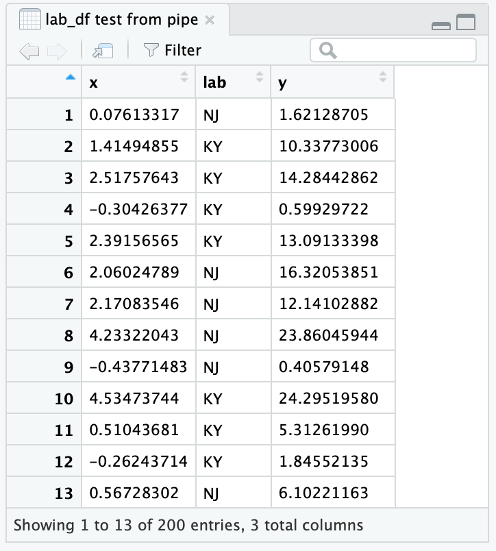
Figure 12.1: RStudio viewer
See Also
See Recipe 12.13, “Revealing the Structure of an Object” for seeing the structure of your variable’s contents.
12.2 Printing the Result of an Assignment
Problem
You are assigning a value to a variable and you want to see its value.
Solution
Simply put parentheses around the assignment:
Discussion
Normally, R inhibits printing when it sees you enter a simple assignment. When you surround the assignment with parentheses, however, it is no longer a simple assignment and so R prints the value. This can be very handy for quick debugging in a script.
See Also
See Recipe 2.1, “Printing Something to the Screen”, for more ways to print things.
12.3 Summing Rows and Columns
Problem
You want to sum the rows or columns of a matrix or data frame.
Discussion
This is a mundane recipe, but it’s so common that it deserves
mentioning. We use this recipe, for example, when producing reports that
include column totals. In this example, daily.prod is a record of this
week’s factory production and we want totals by product and by day:
load(file = './data/daily.prod.rdata')
daily.prod
#>     Widgets Gadgets Thingys
#> Mon     179     167     182
#> Tue     153     193     166
#> Wed     183     190     170
#> Thu     153     161     171
#> Fri     154     181     186
colSums(daily.prod)
#> Widgets Gadgets Thingys
#>     822     892     875
rowSums(daily.prod)
#> Mon Tue Wed Thu Fri
#> 528 512 543 485 521
These functions return a vector. In the case of column sums, we can append the vector to the matrix and thereby neatly print the data and totals together:
12.4 Printing Data in Columns
Problem
You have several parallel data vectors, and you want to print them in columns.
Solution
Use cbind to form the data into columns, then print the result.
Discussion
When you have parallel vectors, it’s difficult to see their relationship if you print them separately:
load(file = './data/xy.rdata')
print(x)
#>  [1] -0.626  0.184 -0.836  1.595  0.330 -0.820  0.487  0.738  0.576 -0.305
print(y)
#>  [1]  1.5118  0.3898 -0.6212 -2.2147  1.1249 -0.0449 -0.0162  0.9438
#>  [9]  0.8212  0.5939
Use the cbind function to form them into columns that, when printed,
show the data’s structure:
print(cbind(x,y))
#>            x       y
#>  [1,] -0.626  1.5118
#>  [2,]  0.184  0.3898
#>  [3,] -0.836 -0.6212
#>  [4,]  1.595 -2.2147
#>  [5,]  0.330  1.1249
#>  [6,] -0.820 -0.0449
#>  [7,]  0.487 -0.0162
#>  [8,]  0.738  0.9438
#>  [9,]  0.576  0.8212
#> [10,] -0.305  0.5939
You can include expressions in the output, too. Use a tag to give them a column heading:
print(cbind(x, y, Total = x + y))
#>            x       y  Total
#>  [1,] -0.626  1.5118  0.885
#>  [2,]  0.184  0.3898  0.573
#>  [3,] -0.836 -0.6212 -1.457
#>  [4,]  1.595 -2.2147 -0.619
#>  [5,]  0.330  1.1249  1.454
#>  [6,] -0.820 -0.0449 -0.865
#>  [7,]  0.487 -0.0162  0.471
#>  [8,]  0.738  0.9438  1.682
#>  [9,]  0.576  0.8212  1.397
#> [10,] -0.305  0.5939  0.289
12.5 Binning Your Data
Problem
You have a vector, and you want to split the data into groups according to intervals. Statisticians call this binning your data.
Solution
Use the cut function. You must define a vector, say breaks, that
gives the ranges of the intervals. The cut function will group your
data according to those intervals. It returns a factor whose levels
(elements) identify each datum’s group:
Discussion
This example generates 1,000 random numbers that have a standard normal distribution. It breaks them into six groups by defining intervals at ±1, ±2, and ±3 standard deviations:
The result is a factor, f, that identifies the groups. The summary
function shows the number of elements by level. R creates names for each
level, using the mathematical notation for an interval:
The results are bell-shaped, which is what we expect from the rnorm function. There are five NA
values, indicating that two values in x fell outside the defined
intervals.
We can use the labels parameter to give nice, predefined names to the
six groups instead of the funky synthesized names:
Now the summary function uses our names:
Binning is useful for summaries such as histograms. But it results in
information loss, which can be harmful in modeling. Consider the extreme
case of binning a continuous variable into two values, high and low.
The binned data has only two possible values, so you have replaced a
rich source of information with one bit of information. Where the
continuous variable might be a powerful predictor, the binned variable
can distinguish at most two states and so will likely have only a
fraction of the original power. Before you bin, we suggest exploring
other transformations that are less lossy.
12.6 Finding the Position of a Particular Value
Problem
You have a vector. You know a particular value occurs in the contents, and you want to know its position.
Solution
The match function will search a vector for a particular value and
return the position:
Here match returns 3, which is the position of 80 within vec.
Discussion
There are special functions for finding the location of the minimum and
maximum values—which.min and which.max, respectively:
See Also
This technique is used in Recipe 11.13, “Finding the Best Power Transformation”.
12.7 Selecting Every nth Element of a Vector
Problem
You want to select every nth element of a vector.
Solution
Create a logical indexing vector that is TRUE for every nth element.
One approach is to find all subscripts that equal zero when taken modulo
n:
Discussion
This problem arises in systematic sampling: we want to sample a dataset
by selecting every nth element. The seq_along(v) function generates
the sequence of integers that can index v; it is equivalent to
1:length(v). We compute each index value modulo n by the expression:
Then we find those values that equal zero:
The result is a logical vector, the same length as v and with TRUE
at every nth element, that can index v to select the desired
elements:
v
#>  [1]  2.325  0.524  0.971  0.377 -0.996 -0.597  0.165 -2.928 -0.848  0.799
v[ seq_along(v) %% n == 0 ]
#> [1]  0.524  0.377 -0.597 -2.928  0.799
If you just want something simple like every second element, you can use
the Recycling Rule in a clever way. Index v with a two-element logical
vector, like this:
If v has more than two elements, then the indexing vector is too short.
Hence, R will invoke the Recycling Rule and expand the index vector to
the length of v, recycling its contents. That gives an index vector
that is FALSE, TRUE, FALSE, TRUE, FALSE, TRUE, and so forth.
Voilà! The final result is every second element of v.
See Also
See Recipe 5.3, “Understanding the Recycling Rule”, for more about the Recycling Rule.
12.8 Finding Minimums or Maximums
Problem
You have two vectors, v and w, and you want to find the minimums or the maximums of pairwise elements. That is, you want to calculate:
min(v1, w1), min(v2, w2), min(v3, w3), …
or:
max(v1, w1), max(v2, w2), max(v3, w3), …
Solution
R calls these the parallel minimum and the parallel maximum. The
calculation is performed by pmin(v,w) and pmax(v,w), respectively:
Discussion
When an R beginner wants pairwise minimums or maximums, a common mistake
is to write min(v,w) or max(v,w). Those are not pairwise operations:
min(v,w) returns a single value, the minimum over all v and w.
Likewise, max(v,w) returns a single value from all of v and w.
The pmin and pmax values compare their arguments in parallel,
picking the minimum or maximum for each subscript. They return a vector
that matches the length of the inputs.
You can combine pmin and pmax with the Recycling Rule to perform
useful hacks. Suppose the vector v contains both positive and negative
values, and you want to reset the negative values to zero. This does the
trick:
By the Recycling Rule, R expands the zero-valued scalar into a vector of
zeros that is the same length as v. Then pmax does an
element-by-element comparison, taking the larger of zero and each
element of v.
Actually, pmin and pmax are more powerful than the Solution
indicates. They can take more than two vectors, comparing all vectors in
parallel.
It is not uncommon to use pmin or pmax to calculate a new variable in a data frame based on multiple fields. Let’s look at a quick example:
df <- data.frame(a = c(1,5,8),
                 b = c(2,3,7),
                 c = c(0,4,9))
df %>%
  mutate(max_val = pmax(a,b,c))
#>   a b c max_val
#> 1 1 2 0       2
#> 2 5 3 4       5
#> 3 8 7 9       9
We can see the new column, max_val, now contains the row-by-row max value from the three input columns.
See Also
See Recipe 5.3, “Understanding the Recycling Rule”, for more about the Recycling Rule.
12.9 Generating All Combinations of Several Variables
Problem
You have two or more variables. You want to generate all combinations of their levels, also known as their Cartesian product.
Discussion
This code snippet creates two vectors—sides represents the two sides
of a coin, and faces represents the six faces of a die (those little
spots on a die are called pips):
We can use expand.grid to find all combinations of one roll of the die
and one coin toss:
expand.grid(faces, sides)
#>      Var1  Var2
#> 1   1 pip Heads
#> 2  2 pips Heads
#> 3  3 pips Heads
#> 4  4 pips Heads
#> 5  5 pips Heads
#> 6  6 pips Heads
#> 7   1 pip Tails
#> 8  2 pips Tails
#> 9  3 pips Tails
#> 10 4 pips Tails
#> 11 5 pips Tails
#> 12 6 pips Tails
Similarly, we could find all combinations of two dice. But we won’t print the output here because it’s 36 lines long:
The result of expand.grid is a data frame. R automatically provides the row names and
column names.
The Solution and the example show the Cartesian product of two vectors,
but expand.grid can handle three or more factors, too.
See Also
If you’re working with strings and want a bit more control over how you bring the combinations together, then you can also use Recipe 7.6, “Generating All Pairwise Combinations of Strings”, to generate combinations.
12.10 Flattening a Data Frame
Problem
You have a data frame of numeric values. You want to process all its elements together, not as separate columns—for example, to find the mean across all values.
Solution
Convert the data frame to a matrix and then process the matrix. This
example finds the mean of all elements in the data frame dfrm:
It is sometimes necessary then to convert the matrix to a vector. In
that case, use as.vector(as.matrix(dfrm)).
Discussion
Suppose we have a data frame, such as the factory production data from Recipe 12.3, “Summing Rows and Columns”:
load(file = './data/daily.prod.rdata')
daily.prod
#>     Widgets Gadgets Thingys
#> Mon     179     167     182
#> Tue     153     193     166
#> Wed     183     190     170
#> Thu     153     161     171
#> Fri     154     181     186
Suppose also that we want the average daily production across all days and products. This won’t work:
mean(daily.prod)
#> Warning in mean.default(daily.prod): argument is not numeric or logical:
#> returning NA
#> [1] NA
The mean function doesn’t really know what to do with a data frame, so it just throws an error. But when you want the average across all
values, first collapse the data frame down to a matrix:
This recipe works only on data frames with all-numeric data. Recall that converting a data frame with mixed data (numeric columns mixed with character columns or factors) into a matrix forces all columns to be converted to characters.
See Also
See Recipe 5.29, “Converting One Structured Data Type into Another”, for more about converting between data types.
12.11 Sorting a Data Frame
Problem
You have a data frame. You want to sort the contents, using one column as the sort key.
Solution
Use the arrange function from the dplyr package:
Here df is a data frame and key is the sort-key column.
Discussion
The sort function is great for vectors but is ineffective for data
frames. Suppose we have the following data frame and we want to sort by month:
load(file = './data/outcome.rdata')
print(df)
#>   month day outcome
#> 1     7  11     Win
#> 2     8  10    Lose
#> 3     8  25     Tie
#> 4     6  27     Tie
#> 5     7  22     Win
The arrange function rearranges the months into ascending
order and returns the entire data frame:
library(dplyr)
arrange(df, month)
#>   month day outcome
#> 1     6  27     Tie
#> 2     7  11     Win
#> 3     7  22     Win
#> 4     8  10    Lose
#> 5     8  25     Tie
After rearranging the data frame, the month column is in ascending
order—just as we wanted. If we want to sort the data in descending order, put a - in front of the column you want to sort by:
arrange(df,-month)
#>   month day outcome
#> 1     8  10    Lose
#> 2     8  25     Tie
#> 3     7  11     Win
#> 4     7  22     Win
#> 5     6  27     Tie
If you want to sort by multiple columns, you can add them to the arrange function. The following example sorts by month first, then by day:
arrange(df, month, day)
#>   month day outcome
#> 1     6  27     Tie
#> 2     7  11     Win
#> 3     7  22     Win
#> 4     8  10    Lose
#> 5     8  25     Tie
Within months 7 and 8, the days are now sorted into ascending order.
12.12 Stripping Attributes from a Variable
Problem
A variable is carrying around old attributes. You want to remove some or all of them.
Solution
To remove all attributes, assign NULL to the variable’s attributes
property:
To remove a single attribute, select the attribute using the attr
function, and set it to NULL:
Discussion
Any variable in R can have attributes. An attribute is simply a
name/value pair, and the variable can have many of them. A common
example is the dimensions of a matrix variable, which are stored in an
attribute. The attribute name is dim and the attribute value is a
two-element vector giving the number of rows and columns.
You can view the attributes of x by printing attributes(x) or
str(x).
Sometimes you want just a number and R insists on giving it attributes. This can happen when you fit a simple linear model and extract the slope, which is the second regression coefficient:
When we print slope, R also prints "x1". That is a name attribute
given by lm to the coefficient (because it’s the coefficient for the
x1 variable). We can see that more clearly by printing the internals
of slope, which reveals a "names" attribute:
It’s easy to strip out all the attributes, after which the slope value becomes simply a number:
attributes(slope) <- NULL    # Strip off all attributes
str(slope)                   # Now the "names" attribute is gone
#>  num -11

slope                        # And the number prints cleanly without a label
#> [1] -11
Alternatively, we could have stripped out the single offending attribute this way:
Warning
Remember that a matrix is a vector (or list) with a
dimattribute. If you strip out all the attributes from a matrix, that will strip away the dimensions and thereby turn it into a mere vector (or list). Furthermore, stripping the attributes from an object (specifically, an S3 object) can render it useless. So remove attributes with care.
See Also
See Recipe 12.13, “Revealing the Structure of an Object”, for more about seeing attributes.
12.13 Revealing the Structure of an Object
Problem
You called a function that returned something. Now you want to look inside that something and learn more about it.
Solution
Use class to determine the thing’s object class:
Use mode to strip away the object-oriented features and reveal the
underlying structure:
Use str to show the internal structure and contents:
Discussion
We are regularly amazed how often we call a function, get something back, and wonder: “What the heck is this thing?” Theoretically, the function documentation should explain the returned value, but somehow we feel better when we can see its structure and contents ourselves. This is especially true for objects with a nested structure: objects within objects.
Let’s dissect the value returned by lm (the linear modeling function)
in the simplest linear regression recipe, Recipe 11.1, “Performing Simple Linear Regression”:
load(file = './data/conf.rdata')
m <- lm(y ~ x1)
print(m)
#>
#> Call:
#> lm(formula = y ~ x1)
#>
#> Coefficients:
#> (Intercept)           x1
#>        15.9        -11.0
Always start by checking the thing’s class. The class indicates if it’s a vector, matrix, list, data frame, or object:
Hmmm. It seems that m is an object of class lm. That may not mean
anything to you, however. But you know that all object classes are built upon
the native data structures (vector, matrix, list, or data frame), so we
use mode to strip away the object facade and reveal the underlying
structure:
Ah-ha! It seems that m is built on a list structure. Now we can use
list functions and operators to dig into its contents. First, we want to
know the names of its list elements:
names(m)
#>  [1] "coefficients"  "residuals"     "effects"       "rank"
#>  [5] "fitted.values" "assign"        "qr"            "df.residual"
#>  [9] "xlevels"       "call"          "terms"         "model"
The first list element is called *"coefficients"*. We could guess those are
the regression coefficients. Let’s have a look:
Yes, that’s what they are. We recognize those values.
We could continue digging into the list structure of m, but that would
get tedious. The str function does a good job of revealing the
internal structure of any variable:
str(m)
#> List of 12
#>  $ coefficients : Named num [1:2] 15.9 -11
#>   ..- attr(*, "names")= chr [1:2] "(Intercept)" "x1"
#>  $ residuals    : Named num [1:30] 36.6 58.6 112.1 -35.2 -61.7 ...
#>   ..- attr(*, "names")= chr [1:30] "1" "2" "3" "4" ...
#>  $ effects      : Named num [1:30] -73.1 69.3 93.9 -31.1 -66.3 ...
#>   ..- attr(*, "names")= chr [1:30] "(Intercept)" "x1" "" "" ...
#>  $ rank         : int 2
#>  $ fitted.values: Named num [1:30] 25.69 13.83 -1.55 28.25 16.74 ...
#>   ..- attr(*, "names")= chr [1:30] "1" "2" "3" "4" ...
#>  $ assign       : int [1:2] 0 1
#>  $ qr           :List of 5
#>   ..$ qr   : num [1:30, 1:2] -5.477 0.183 0.183 0.183 0.183 ...
#>   .. ..- attr(*, "dimnames")=List of 2
#>   .. .. ..$ : chr [1:30] "1" "2" "3" "4" ...
#>   .. .. ..$ : chr [1:2] "(Intercept)" "x1"
#>   .. ..- attr(*, "assign")= int [1:2] 0 1
#>   ..$ qraux: num [1:2] 1.18 1.02
#>   ..$ pivot: int [1:2] 1 2
#>   ..$ tol  : num 1e-07
#>   ..$ rank : int 2
#>   ..- attr(*, "class")= chr "qr"
#>  $ df.residual  : int 28
#>  $ xlevels      : Named list()
#>  $ call         : language lm(formula = y ~ x1)
#>  $ terms        :Classes 'terms', 'formula'  language y ~ x1
#>   .. ..- attr(*, "variables")= language list(y, x1)
#>   .. ..- attr(*, "factors")= int [1:2, 1] 0 1
#>   .. .. ..- attr(*, "dimnames")=List of 2
#>   .. .. .. ..$ : chr [1:2] "y" "x1"
#>   .. .. .. ..$ : chr "x1"
#>   .. ..- attr(*, "term.labels")= chr "x1"
#>   .. ..- attr(*, "order")= int 1
#>   .. ..- attr(*, "intercept")= int 1
#>   .. ..- attr(*, "response")= int 1
#>   .. ..- attr(*, ".Environment")=<environment: R_GlobalEnv>
#>   .. ..- attr(*, "predvars")= language list(y, x1)
#>   .. ..- attr(*, "dataClasses")= Named chr [1:2] "numeric" "numeric"
#>   .. .. ..- attr(*, "names")= chr [1:2] "y" "x1"
#>  $ model        :'data.frame':   30 obs. of  2 variables:
#>   ..$ y : num [1:30] 62.25 72.45 110.59 -6.94 -44.99 ...
#>   ..$ x1: num [1:30] -0.8969 0.1848 1.5878 -1.1304 -0.0803 ...
#>   ..- attr(*, "terms")=Classes 'terms', 'formula'  language y ~ x1
#>   .. .. ..- attr(*, "variables")= language list(y, x1)
#>   .. .. ..- attr(*, "factors")= int [1:2, 1] 0 1
#>   .. .. .. ..- attr(*, "dimnames")=List of 2
#>   .. .. .. .. ..$ : chr [1:2] "y" "x1"
#>   .. .. .. .. ..$ : chr "x1"
#>   .. .. ..- attr(*, "term.labels")= chr "x1"
#>   .. .. ..- attr(*, "order")= int 1
#>   .. .. ..- attr(*, "intercept")= int 1
#>   .. .. ..- attr(*, "response")= int 1
#>   .. .. ..- attr(*, ".Environment")=<environment: R_GlobalEnv>
#>   .. .. ..- attr(*, "predvars")= language list(y, x1)
#>   .. .. ..- attr(*, "dataClasses")= Named chr [1:2] "numeric" "numeric"
#>   .. .. .. ..- attr(*, "names")= chr [1:2] "y" "x1"
#>  - attr(*, "class")= chr "lm"
Notice that str shows all the elements of m and then recursively
dumps each element’s contents and attributes. Long vectors and lists are
truncated to keep the output manageable.
There is an art to exploring an R object. Use class, mode, and str
to dig through the layers. We have found that often str tells you everything you want to know…and sometimes a lot more.
12.14 Timing Your Code
Problem
You want to know how much time is required to run your code. This is useful, for example, when you are optimizing your code and need “before” and “after” numbers to measure the improvement.
Solution
The tictoc package contains a very easy way to time and label chunks of code. The tic function starts a timer and the toc function stops the timer and reports the
execution time:
The output is the execution time in seconds.
Discussion
Suppose we want to know the time required to generate 10,000,000 random normal numbers and sum them together:
library(tictoc)
tic('making big numbers')
total_val <- sum(rnorm(1e7))
toc()
#> making big numbers: 0.88 sec elapsed
The toc function returns the message set in tic along with the runtime in seconds.
If you assign the result of toc to an object, you can have access to the underlying start time, finish time, and message:
tic('two sums')
sum(rnorm(10000000))
#> [1] -84.1
sum(rnorm(10000000))
#> [1] -3899
toc_result <- toc()
#> two sums: 1.586 sec elapsed

print(toc_result)
#> $tic
#> elapsed
#>    3.11
#>
#> $toc
#> elapsed
#>    4.69
#>
#> $msg
#> [1] "two sums"
If you want to report the results in minutes (or hours!), you can use the elements of the output to get at the underlying start and finish times:
print(paste('the code ran in',
            round((toc_result$toc -  toc_result$tic) / 60, 4),
            'minutes'))
#> [1] "the code ran in 0.0264 minutes"
You can accomplish the same thing using just Sys.time calls but without the convenience of labeling and clarity of syntax provided by toctoc:
12.15 Suppressing Warnings and Error Messages
Problem
A function is producing annoying error messages or warning messages. You don’t want to see them.
Solution
Surround the function call with suppressMessage(…) or
suppressWarnings(…):
Discussion
The Augmented Dickey–Fuller Test, adf.test, is a popular time series function. However, it produces an
annoying warning message, shown here at the bottom of the output, when
the p-value is below 0.01:
library(tseries)
#> Registered S3 method overwritten by 'xts':
#>   method     from
#>   as.zoo.xts zoo
#> Registered S3 method overwritten by 'quantmod':
#>   method            from
#>   as.zoo.data.frame zoo
load(file = './data/adf.rdata')
results <- adf.test(x)
#> Warning in adf.test(x): p-value smaller than printed p-value
Fortunately, we can muzzle the function by calling it inside
suppressWarnings(…):
Notice that the warning message disappeared. The message is not entirely
lost because R retains it internally. We can retrieve the message at our
leisure by using the warnings function:
Some functions also produce “messages” (in R terminology), which are
even more benign than warnings. Typically, they are merely informative
and not signals of problems. If such a message is annoying you, call the
function inside suppressMessages(...), and the message will
disappear.
See Also
See the options function for other ways to control the reporting of
errors and warnings.
12.16 Taking Function Arguments from a List
Problem
Your data is captured in a list structure. You want to pass the data to a function, but the function does not accept a list.
Solution
In simple cases, convert the list to a vector. For more complex cases,
the do.call function can break the list into individual arguments and
call your function:
Discussion
If your data is in a vector, life is simple and most R functions work as expected:
If your data is captured in a list, some functions complain and return a useless result, like this:
numbers <- list(1, 3, 5, 7, 9)
mean(numbers)
#> Warning in mean.default(numbers): argument is not numeric or logical:
#> returning NA
#> [1] NA
The numbers list is a simple, one-level list, so we can just convert
it to a vector and call the function:
The big headaches come when you have multilevel list structures: lists within lists. These can occur within complex data structures. Here is a list of lists in which each sublist is a column of data:
my_lists <-
  list(col1 = list(7, 8),
       col2 = list(70, 80),
       col3 = list(700, 800))
my_lists
#> $col1
#> $col1[[1]]
#> [1] 7
#>
#> $col1[[2]]
#> [1] 8
#>
#>
#> $col2
#> $col2[[1]]
#> [1] 70
#>
#> $col2[[2]]
#> [1] 80
#>
#>
#> $col3
#> $col3[[1]]
#> [1] 700
#>
#> $col3[[2]]
#> [1] 800
Suppose we want to form this data into a matrix. The cbind function is
supposed to create data columns, but it gets confused by the list
structure and returns something useless:
If we unlist the data then we just get one big, long column, which is not what we are after either:
cbind(unlist(my_lists))
#>       [,1]
#> col11    7
#> col12    8
#> col21   70
#> col22   80
#> col31  700
#> col32  800
The solution is to use do.call, which splits the list into individual
items and then calls cbind on those items:
Using do.call in that way is functionally identical to calling cbind
like this:
cbind(my_lists[[1]], my_lists[[2]], my_lists[[3]])
#>      [,1] [,2] [,3]
#> [1,] 7    70   700
#> [2,] 8    80   800
Be careful if the list elements have names. In that case, do.call
interprets the element names as names of parameters to the function,
which might cause trouble.
This recipe presents the most basic use of do.call. The function is
quite powerful and has many other uses. See the help page for more
details.
See Also
See Recipe 5.29, “Converting One Structured Data Type into Another”, for converting between data types.
12.17 Defining Your Own Binary Operators
Problem
You want to define your own binary operators, making your R code more streamlined and readable.
Solution
R recognizes any text between percent signs (%…%) as a binary
operator. Create and define a new binary operator by assigning a
two-argument function to it.
Discussion
R contains an interesting feature that lets you define your own binary
operators. Any text between two percent signs (%…%) is
automatically interpreted by R as a binary operator. R predefines
several such operators, such as %/% for integer division, %*% for
matrix multiplication, and the pipe %>% in the magrittr package.
You can create a new binary operator by assigning a function to it. This
example creates an operator, %+-%:
The expression x %+-% m calculates x ± m. Here it calculates 100 ±
(1.96 × 15), the two-standard-deviation range of a standard IQ test:
Notice that we quote the binary operator when defining it but not when using it.
The pleasure of defining your own operators is that you can wrap commonly used operations inside a succinct syntax. If your application frequently concatenates two strings without an intervening blank, then you might define a binary concatenation operator for that purpose:
'%+%' <- function(s1, s2)
  paste(s1, s2, sep = "")
"Hello" %+% "World"
#> [1] "HelloWorld"
"limit=" %+% round(qnorm(1 - 0.05 / 2), 2)
#> [1] "limit=1.96"
A danger of defining your own operators, however, is that the code becomes less portable to other environments. Bring the definitions along with the code in which they are used; otherwise, R will complain about undefined operators.
All user-defined operators have the same precedence and are listed
collectively in Table 2.1 as %any%. Their
precedence is fairly high: higher than multiplication and division but
lower than exponentiation and sequence creation. As a result, it’s easy
to misexpress yourself. If we omit parentheses from the %+-%
example, we get an unexpected result:
R interpreted the expression as (100 %+-% 1.96) * 15.
See Also
See Recipe 2.11, “Getting Operator Precedence Right”, for more about operator precedence and Recipe 15.3, “Defining a Function”, for how to define a function.
12.18 Suppressing the Startup Message
Problem
When you run R from a command prompt or shell script, you are tired of seeing R’s verbose startup message.
Solution
Use the --quiet command-line option when you start R from the command line or shell script.
Discussion
The startup message from R is handy for beginners because it contains useful information about the R project and getting help. But the novelty wears off pretty quickly—especially if you start R from a shell prompt to use it as a calculator throughout the day. This is not particularly helpful if you’re using R only from RStudio.
If you start R from the shell prompt, use the --quiet option to hide
the startup message:
On a Linux or Mac box, you could alias R like this from the shell so you never see the startup message:
12.19 Getting and Setting Environment Variables
Problem
You want to see the value of an environment variable, or you want to change its value.
Solution
Use the Sys.getenv function to see values. Use Sys.putenv to change
them:
Discussion
Environment variables are often used to configure and control software. Each process has its own set of environment variables, which are inherited from its parent process. You sometimes need to see the environment variable settings for your R process in order to understand its behavior. Likewise, you sometimes need to change those settings to modify that behavior.
A common use case is to store a username or password for use in accessing a remote database or cloud service. It’s a really bad idea to store passwords in plain text in a project script. One way to avoid storing passwords in your script is to set an environment variable containing your password when R starts.
To ensure our password and username are available at every R login, we can add calls to Sys.setenv in our .Rprofile file in our home directory. The .Rprofile is an R script that is run every time R starts.
We can add the following to our .Rprofile:
Then we can then fetch and use the environment variables in a script to log into an Amazon Redshift database, for example:
See Also
See Recipe 3.16, “Customizing R Startup”, for more about changing configuration at startup.
12.20 Use Code Sections
Problem
You’ve got a long script and you’re finding it difficult to navigate from one section of code to the next.
Solution
Code sections provide section dividers in an outline pane on the side of your editor. To use code sections, simply start a comment with # and then end the comment with ---- or #### or ====:
In the RStudio editor window you can see the outline on the righthand side of Figure 12.2.
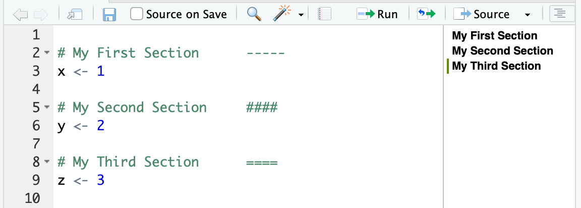
Figure 12.2: Code sections
Discussion
Code sections are just a specially formatted type of R comment since they start with the # symbol. If you open your code with any editor other than RStudio, they are treated simply as code comments. But RStudio sees these specially formatted code comments as section headers and creates a helpful outline in the side of the editor.
The first time you use code sections, you may need to click the outline icon to the right of the Source button in order to show the outline.
If you are writing R Markdown instead of a *.R script, your Markdown headings and subheadings will show up in the outline pane, making navigating your document much easier.
See Also
See Recipe 16.4, “Inserting Document Headings”, for using section headings in R Markdown documents.
12.21 Executing R in Parallel Locally
Problem
You have code that takes a while to run and you would like to speed it up by using more of the cores on your local computer.
Solution
The easiest solution to get up and running with is to use the furrr package, which in turn uses the future package to provide parallel processing via functions that feel like those from purrr except that they operate in parallel.
To use furrr we downloaded the latest development version from GitHub because the package is still under active development as of this writing:
To use furrr to parallelize our code, we call the furrr::future_map in place of the purrr::map function we discussed in Recipe 6.1, “Applying a Function to Each List Element”. But first we have to tell furrr how we want to parallelize. In this case we want a multiprocess parallel process that uses all our local processors. So we set that up by calling plan(multiprocess). Then we can apply a function to every element in our list using future_map:
Discussion
Let’s do an example simulation to illustrate parallelization. A classic stochastic simulation is to draw random points inside of a 2 x 2 box and see how many points fall within one unit from the center of the box. The ratio of points inside the box / total points then multiplied by 4 is a good estimate of pi. The following function takes one input, n_iterations, which is the number of random points to simulate. Then it returns the resulting average estimate of pi:
simulate_pi <- function(n_iterations) {
  rand_draws <- matrix(runif(2 * n_iterations, -1, 1), ncol = 2)
  num_in <- sum(sqrt(rand_draws[, 1]**2 + rand_draws[, 2]**2) <= 1)
  pi_hat <- (num_in / n_iterations) * 4
  return(pi_hat)
}
simulate_pi(1000000)
#> [1] 3.14
As you can see, even with 1,000,000 simulations the result is only accurate out to a couple of decimal points. This is not a very efficient way to estimate pi, but it works for our illustration.
For the purpose of comparison later, let’s run 200 runs of this pi simulator where each run has 5,000,000 simulated points.
We’ll do this by creating a list with 200 elements, each of which is the value 5,000,000, which we will pass to simulate_pi.
We’ll time the code with the tictoc package:
library(purrr)  # for `map`
library(tictoc) # for timing our code

draw_list <- as.list(rep(5000000, 200))

tic("simulate pi - single process")
sims_list <- map(draw_list, simulate_pi)
toc()
#> simulate pi - single process: 131.861 sec elapsed

mean(unlist(sims_list))
#> [1] 3.14
That runs in less than two minutes and gives an estimate of pi based on a billion simulation (5m x 200).
Now let’s take the exact same R function, simulate_pi, and run it through future_map to run it in parallel:
library(furrr)
#> Loading required package: future
#>
#> Attaching package: 'future'
#> The following object is masked from 'package:tseries':
#>
#>     value
plan(multiprocess)

tic("simulate pi - parallel")
sims_list <- future_map(draw_list, simulate_pi)
toc()
#> simulate pi - parallel: 93.005 sec elapsed
mean(unlist(sims_list))
#> [1] 3.14
The preceding example was run on a MacBook Pro with four physical cores and two virtual cores per physical core. When you’re running code in parallel the best-case scenario is that the runtime is reduced by 1/(number of physical cores). With four physical cores you can see the parallel runtime is much faster than the single-threaded version, but not quite one-fourth the runtime of the single-threaded version. There is always some overhead from moving the data around, so you will never experience the best-case scenario. And the more data each iteration produces, the less speed improvement you will experience from parallelization.
See Also
See Recipe @ref(recipe-parallel_remote), “Executing R in Parallel Remotely”
12.22 Executing R in Parallel Remotely
Problem
You have access to a number of remote machines and you would like to run your code in parallel across them all.
Solution
Running code in parallel across multiple machines can be tricky to set up initially. However, if we start with a few key prerequisites in place, the process has a much higher probability of success.
Starting prerequisites:
- You can
sshfrom your main machine to each remote node without a password using previously generated SSH keys. - The remote nodes all have R installed (ideally the same version of R).
- Paths are set such that you can run
Rscriptfrom SSH. - The remote nodes have the package
furrrinstalled (which in turn installsfuture). - The remote nodes already have all the packages installed on which your distributed code depends.
Once you have worker nodes that are set up and ready to go, you can create a cluster by calling makeClusterPSOCK from the future package. Then use the resulting cluster with the furrr function future_map:
Discussion
Suppose we have two big Linux machines named von-neumann12 and von-neumann15 that we can use to run numerical models. These machines meet the criteria just listed, so they are good candidates to be our backend for a furrr/future cluster. Let’s do the same pi simulation we did in the prior recipe using the simulate_pi function:
library(tidyverse)
library(furrr)
library(tictoc)

my_workers <- c('von-neumann12','von-neumann15')

cl <- makeClusterPSOCK(
  workers = my_workers,
  rscript = '/home/anaconda2/bin/Rscript',  #yours may differ
  verbose=TRUE
)

draw_list <- as.list(rep(5000000, 200))

plan(cluster, workers = cl)

tic('simulate pi - parallel map')
sims_list_parallel <- draw_list %>%
  future_map(simulate_pi)
toc()
#> simulate pi - parallel map: 116.986 sec elapsed

mean(unlist(sims_list_parallel))
#> [1] 3.14167
This is ~8.5 million sims per second.
The two nodes in our ad hoc cluster each have 32 processors and 128GB of RAM. But if you compare the runtime of the preceding code with the runtime of the prior recipe run on a humble MacBook Pro, you’ll notice that the MacBook executed the code in about the same time as the multi-CPU Linux cluster with 64 total processors! This unintuitive surprise happens because the preceding code runs only on one CPU per cluster node. So, as a result, it uses only two CPUs, while the MacBook example uses all four of its CPUs.
So how do we run parallel code on a cluster and have each node also run in parallel across multiple CPU cores? To do that we need to make three changes to our code:
- Create a nested parallel plan that uses both
clusterandmultiprocess. - Create an input list that is a nested list. Each cluster machine will get from the main list an item that contains sublist items that it can process in parallel across all its CPUs.
- Call
future_maptwice using a nested call. The outerfuture_mapwill parallelize items across the cluster nodes, and then the inner call will parallelize across the CPUs.
To created the nested parallel plan, we will create a multipart plan by passing a list of two plans to the plan function like this:
plan(list(tweak(cluster, workers = cl), multiprocess))The second change is to create the nested list to iterate on. We can do that by using the split command and passing it our prior list followed by a vector of 1:4 like so:
split(draw_list, 1:4)This will break the initial list into four sublists. So our resulting list will have four elements. Each sublist will have 50 inputs for our final simulate_pi function.
The third change to our code is to create a nested future_map call that will pass each of our four list elements to the worker nodes, which subsequently will iterate over the elements of each sublist. We create that nested function like this:
future_map(draw_list, ~future_map(.,simulate_pi))The ~ sets up R to expect an anonymous function inside the first future_map call, and the . tells R where to put the list element. The anonymous function in this example is a separate call to future_map that gets executed on each node.
Here’s all three changes integrated into code:
# nested parallel plan. The first part of the plan is the cluster call
# followed by the multiprocess
plan(list(tweak(cluster, workers = cl), multiprocess))

# break the draw_list into a nested list with fewer elements
draw_list_nested <- split(draw_list, 1:4)

tic('simulate pi - parallel nested map')
sims_list_nested_parallel <- future_map(draw_list_nested, ~future_map(.,simulate_pi))
toc()
#> simulate pi - parallel nested map: 15.964 sec elapsed
mean(unlist(sims_list_nested_parallel))
#> [1] 3.14158
You can see the runtime decreased substantially from the prior example. Although with 32 processors on each node, we’re not seeing a 32x improvement in runtime. This is because we’re passing only 50 sets of simulations to each node. Each node runs 32 sets of simulations in the first pass but only 18 in the second pass, leaving half the CPUs idle.
Let’s keep the CPUs a little busier by increasing our total simulations from 1 billion to 25 billion. Then we’ll break them into 500 work blocks to be spread to the two worker nodes:
draw_list <- as.list(rep(5000000, 5000))
draw_list_nested <- split(draw_list, 1:50)

plan(list(tweak(cluster, workers = cl), multiprocess))

tic('simulate pi - parallel nested map')
sims_list_nested_parallel <- future_map(draw_list_nested, ~future_map(.,simulate_pi))
toc()
#> simulate pi - parallel nested map: 260.532 sec elapsed
mean(unlist(sims_list_nested_parallel))
#> [1] 3.14157
This gives us ~ 96 million sims per second.
See Also
The future package has multiple excellent vignettes. To better understand the nested plan call, start with vignette('future-3-topologies',package = 'future').
Further info about furrr can be found at its GitHub page.