16 R Markdown and Publishing
Introduction
While R by itself is an incredibly powerful tool for data analysis and visualization, almost all of us, after we do analysis, will need to communicate the results to others. We may do that with published papers, blog posts, PowerPoint presentations, or books. R Markdown is the tool that helps us go from R analysis and visualization all the way to publishable documents.
R Markdown is a package (as well as an ecosystem of tools) that allows us to add R code to a plain-text file with some Markdown formatting. The document can then be rendered into many different output formats including PDF, HTML, Microsoft Word, and Microsoft PowerPoint. At rendering, also called knitting, the R code is run and the resulting output and figures are placed in the final document.
In this chapter we’ll give you recipes to get you started creating R Markdown documents. After you go through these recipes, one of the best ways to learn more about R Markdown is by looking at the source files and final output of other people’s R Markdown work. The book you are reading was itself written in R Markdown. You can see the source to this book on GitHub.
In addition, Yihui Xie, J. J. Allaire, and Garrett Grolemund have written R Markdown: The Definitive Guide and also made the source R Markdown available on GitHub.
Many other books written with R Markdown have been made freely available online.
We mentioned that R Markdown is an ecosystem as well as a package. There are specialized packages to extend R Markdown for blogging (blogdown), for books (bookdown), and for making gridded dashboards (flexdashboard). The initial package in the ecosystem is called knitr, and we still call the process of turning R Markdown into a final format knitting the document. There are many output formats supported by the R Markdown ecosystem and covering them all is unreasonable. So in this book we’ll stick primarily to four common output formats: HTML, LaTeX, Microsoft Word, and Microsoft PowerPoint.
The RStudio IDE contains many helpful features for creating and editing R Markdown documents. While we’ll make use of those features in the following recipes, R Markdown is not dependent on RStudio in order to be useful. It’s possible to edit plain-text R Markdown files with your favorite text editor and then knit the document using R’s command-line interface. However, the RStudio tools are so helpful that we’ll illustrate them extensively.
16.1 Creating a New Document
Problem
You want to create a new R Markdown document to tell your data story.
Solution
The easiest way to create a new R Markdown document is using the File → New File → R Markdown… menu choice in RStudio IDE (see Figure ??).
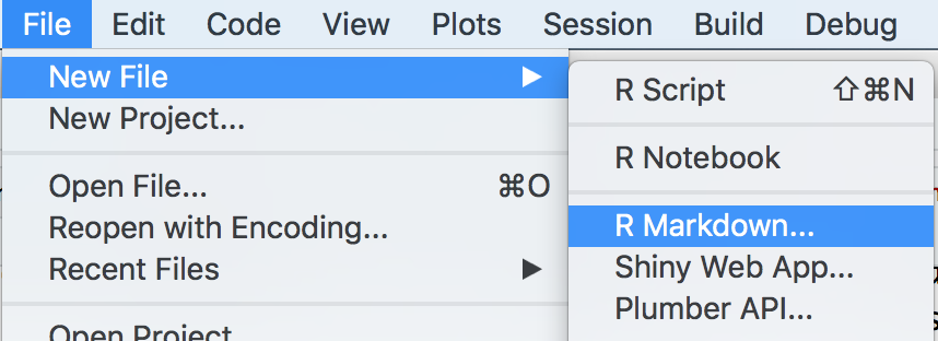
Figure 16.1: Create New R Markdown Document
Selecting “R Markdown…” will lead to the New R Markdown dialog window, where you can choose the type of desired output document you would like to create (see Figure ??). The default option is HTML, which is a good choice if you want to publish your work online or in an email, or if you haven’t made up your mind yet about how you’d like to output your final document. Changing to a different format later is typically as easy as chaining one line of text in the document, or a few clicks in the IDE.
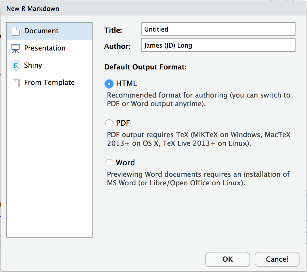
Figure 16.2: New R Markdown Document options
After you make your selection and click OK, you’ll get an R Markdown template with some metadata and example text (see Figure ??).
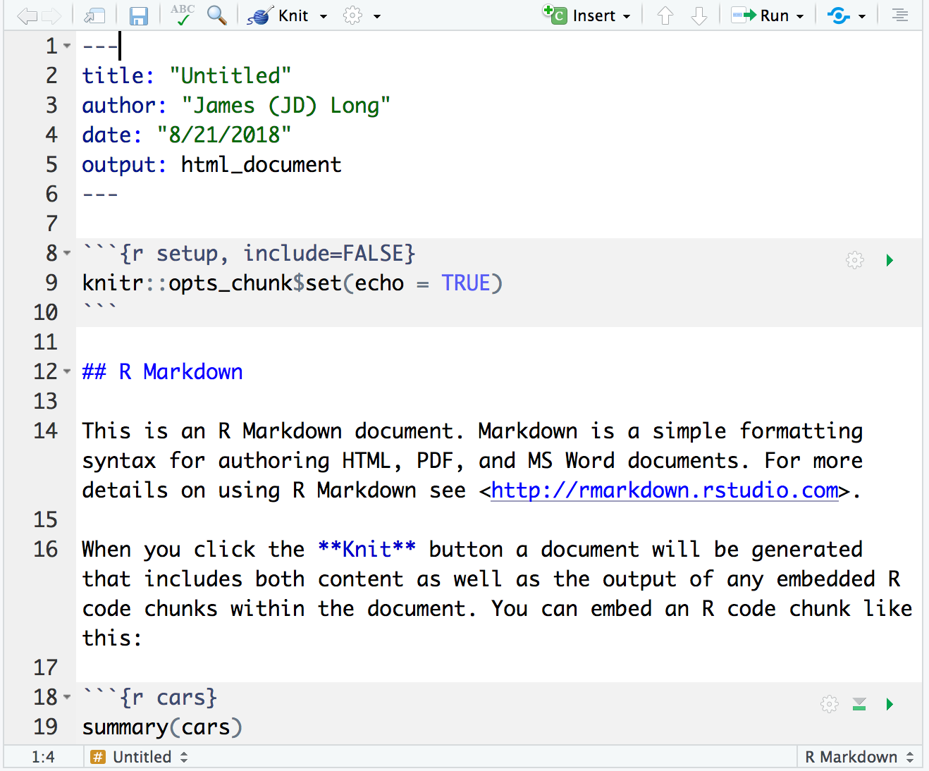
Figure 16.3: New R Markdown document
Discussion
R Markdown documents are plain-text files. The shortcut just outlined is the fastest way to get a template for creating a new R Markdown text document. Once you have the template you can edit the text, alter the R code, and change anything you want. The other recipes in this chapter deal with the types of things you will likely want to do in your R Markdown document. But if you just want to see what some output looks like, click on the Knit button in the RStudio IDE and your R Markdown document will be rendered into your desired output format.
16.2 Adding a Title, Author, or Date
Problem
You want to alter the title, author, or date of your document.
Solution
At the top of an R Markdown document is a block of specially formatted text that starts and ends with ---.
This block contains important metadata about your document.
In this block, you can set the title, author, and date.
---
title: "Your Title Here"
author: "Your Name Here"
date: "12/31/9999"
output: html_document
---
You can also set the output format (e.g., output: html_document).
We’ll discuss the different output formats later in the recipes that cover specific output formats.
Discussion
When you knit your R Markdown document to create your output, R will run each chunk, create Markdown (not R Markdown) for each chunk’s output, and pass the full Markdown document to Pandoc. Pandoc is the software that creates your final output document from the intermediate Markdown. Most of the time, you don’t even need to think about the steps unless you’re having a problem knitting your document.
The text at the top of your R Markdown document between the --- marks is in a format called YAML (Yet Another Markup Language).
This chunk is used to pass metadata to the Pandoc software that builds your output document.
The fields title, author, and date are read by Pandoc and inserted at the top of most output document formats.
The way these values are formatted and inserted into the output document is a function of the template used for output. The default templates for HTML, PDF, and Microsoft Word each format the title, author, and date fields similarly (see Figure (headerblock)).

Figure 16.4: Header illustration
You can add other key/value pairs into the YAML header, but if your template is not configured to use these values, they are ignored.
See Also
For information on creating your own templates, see Chapter 17, “Document Templates,” in R Markdown: The Definitive Guide.
16.3 Formatting Document Text
Problem
You want to format the text of your document, such as putting text into italics or bold.
Solution
The body of an R Markdown document is plain text and allows formatting using Markdown notation. You’ll likely want to add formatting, such as making text bold or italic. You’ll also want to add section headers, lists, and tables, which will be covered in later recipes. All of these options can be accomplished through Markdown.
Table 16.1 shows a brief summary of some of the most common formatting syntax.
| Markdown | Output |
|---|---|
plain text |
plain text |
*italics* |
italics |
**bold** |
bold |
`code` |
code |
sub~script~ |
subscript |
super^script^ |
superscript |
~~strikethrough~~ |
|
endash: -- |
endash: – |
emdash: --- |
emdash: — |
See Also
RStudio publishes a handy reference sheet.
See also recipes for inserting various structures, such as Recipes 16.4, “Inserting Document Headings”, 16.5, “Inserting a List”, and 16.9, “Inserting a Table”.
16.4 Inserting Document Headings
Problem
Your R Markdown document needs section headings.
Solution
You can insert section headings by starting a line with the # (hash) character.
Use one hash character for the top level, two for the second level, and so on.
# Level 1 Heading
## Level 2 Heading
### Level 3 Heading
#### Level 4 Heading
##### Level 5 Heading
###### Level 6 Heading
Discussion
Markdown and HTML both support up to six heading levels, so that’s what’s also supported in R Markdown. In R Markdown (and Markdown in general) the formatting does not include specific font details. The formatting communicates only what formatting class to apply to text. The specifics of each class are defined by the output format and the template used by each output format.
16.5 Inserting a List
Problem
You want to include a bulleted or numbered list in your document.
Solution
To create a bulleted list, start each line with an asterisk (*) like so:
* first item
* second item
* third item
To create a numbered list, start each line with 1. as follows:
1. first item
1. second item
1. third item
R Markdown will replace the 1. prefixes with the sequence 1., 2., 3., and so on.
The rules for lists are a bit strict:
- There must be a blank line before the list.
- There must be a blank line after the list.
- There must be a space character after the leading asterisk.
Discussion
The syntax for lists is simple, but watch out for “the rules” given in the Solution. If you violate even one, the output will be gobbledygook.
An important feature of lists is that they allow sublists. This bulleted list has three subitems:
* first item
   * first subitem
   * second subitem
   * third subitem
* second item
which produces this output:
- first item
- first subitem
- second subitem
- third subitem
- second item
Again, there is an important rule: the sublists must be indented by two, three, or four spaces relative to the level above. No more, no less—otherwise, chaos will ensue.
The Solution recommends using the prefix 1. to identify numbered lists.
You can also use a. and i. which will produce lowercase letters and roman numeral sequences, respectively.
That’s handy for formatting sublists.
1. first item
1. second item
   a. subitem 1
   a. subitem 2
      i. sub-subitem 1
      i. sub-subitem 2
   a. subitem 2
1. third item- first item
- second item
- subitem 1
- subitem 2
- sub-subitem 1
- sub-subitem 2
- subitem 2
- third item
See Also
The syntax for lists is more flexible and feature-laden than described here. See the reference material for details, such as the Pandoc Markdown guide.
16.6 Showing Output from R Code
Problem
You want to execute some R code and show the results in the output document.
Solution
You can insert R code in an R Markdown document. It will be executed and the output included in the final document.
There are two ways to insert the code. For small bits of code, include them inline between two tic marks (```), such as:
The square root of pi is `r sqrt(pi)`. which results in this output:
The square root of pi is 1.772.
For larger blocks of code, define a code chunk
by placing the block between matching triple tic marks (```).
Note the little {r} after the first triple tic marks,
alerting R Markdown that we want it to execute the code.
Discussion
Embedding R code into your document is the most powerful feature of R Markdown. In fact, without that feature, R Markdown would just be plain old Markdown.
Inline R, described first in the Solution, is useful for pulling in small bits of information directly into the text of a report, information such as dates, times, or the results of small calculations.
Code chunks are for doing the heavy lifting.
By default, the code chunk is shown in the text, and the results are displayed directly under the code.
The results are preceded by a prefix, which defaults to a double hash tag: ##.
If we had this code chunk in a source R Markdown document:
it would produce this output:
Conveniently, having the results preceded by the ## allows the reader to paste
the code and results into their own R session and execute the code.
R will ignore the results because they look like comments.
The small {r} after the tic marks is important because R Markdown allows
code blocks from other languages, too, such as Python or SQL.
If you work in a multilanguage environment, this is a very powerful feature.
See the R Markdown documentation for details.
See Also
Recipe 16.7, “Controlling Which Code and Results Are Shown”
“Other Language Engines” from R Markdown: The Definitive Guide.
16.7 Controlling Which Code and Results Are Shown
Problem
Your document contains chunks of R code. You want to control what’s shown in the final document: only the results, only the code, or neither.
Solution
Code blocks support several options that control what appears in the final document.
Set the options at the top of the block. For example, this block has echo set to FALSE.
See the Discussion for a table of available options.
Discussion
There are many display options,
such as echo, which controls whether the code itself appears in the final output,
or eval, which controls whether or not the code is evaluated (executed).
A few of the most popular options are listed in Table 16.2.
| Chunk option | Executes code | Shows code | Shows output text | Shows figures |
|---|---|---|---|---|
results='hide' |
X | X | X | |
include=FALSE |
X | |||
echo=FALSE |
X | X | X | |
fig.show='hide' |
X | X | X | |
eval=FALSE |
X |
You can mix and match combinations of options to get the results you’re after. Some common use cases are:
- You want the code’s output to appear, but not the code itself:
echo=FALSE - You want the code to appear, but not be executed:
eval=FALSE - You want to execute the code for its side effects (e.g., loading packages or loading data),
but neither the code nor any incidental output should appear:
include=FALSE
We often use include=FALSE for the first code chunk of an R Markdown document,
where we are calling library, initializing variables, and doing other housekeeping tasks
whose incidental output is just an annoyance.
In addition to the output options just described, there are several options that control handling of the error messages, warning messages, and informational messages generated by your code:
error=TRUEallows your document to build completely even if there is an error in the code chunk. This is helpful when you’re creating a document where you specifically want to see the error in the output. The default iserror=FALSE.warning=FALSEsuppresses warning messages. The default iswarning=TRUE.message=FALSEsuppresses informational messages. This is handy when your code uses chatty packages that produce messages while loading. The default ismessage=TRUE.
See Also
The R Markdown cheat sheet from RStudio lists many available options.
The author of knitr, Yihui Xie, documented the options on his website.
16.8 Inserting a Plot
Problem
You want to insert a plot into your output document.
Solution
Simply create a code chunk that creates the plot, and insert that chunk into your R Markdown document. R Markdown will capture the plot and insert it into your output document.
Discussion
Here is an R Markdown code chunk that creates a ggplot plot called gg,
then “prints” it:
Recall that print(gg) renders the plot.
If we insert this code chunk into an R Markdown document,
R Markdown will capture the result and insert it into the output,
which looks something like this:

Figure 16.5: Example ggplot in R Markdown
The resulting plot is shown in Figure 16.5.
Almost any plot we can produce in R can be rendered into the output document.
We have some control over the rendered results using options in the code block,
such as setting the size, resolution, and format of the output.
Let’s look at some examples using the gg plot object we created earlier.
We can shrink the output using out.width:
which results in Figure 16.6:

Figure 16.6: Small-width plot
Or we can enlarge the output to the full width of the page.
which results in Figure 16.7:
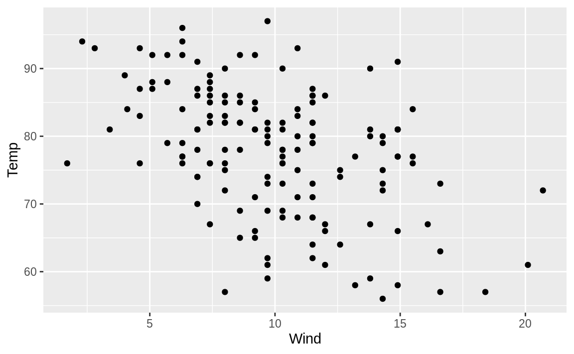
Figure 16.7: Large-width plot
Some common output settings to use with graphics are:
out.widthandout.height: Size of the output figure as a percentage of the page size.dev: The R graphical device used to create the figure. The default is'png'for HTML output and'pdf'for LaTeX output. You can also use'jpg'or'svg', for example.fig.cap: Figure caption.fig.align: Alignment of plot:'left','center', or'right'.
Let’s use these settings to create a figure with 50% width, 20% height, a caption, and left alignment:
```{r out.width='50%', out.height='20%', fig.cap='Temperature versus wind speed', fig.align='left'}
print(gg)
```
This produces Figure 16.8.

Figure 16.8: Temperature vs. Wind Speed
16.9 Inserting a Table
Problem
You want to insert a nicely formatted table into your document.
Solution
Layout the contents in a text table, using the pipe character (|) to separate columns.
Use dashes to “underline” column headings.
R Markdown will format that into attractive output.
For example, this input:
| Stooge | Year | Hair?           |
|--------|------|-----------------|
| Moe    | 1887 | Yes             |
| Larry  | 1902 | Yes             |
| Curly  | 1903 | No (ironically) |
will produce this output.
| Stooge | Year | Hair? |
|---|---|---|
| Moe | 1887 | Yes |
| Larry | 1902 | Yes |
| Curly | 1903 | No (ironically) |
You must place a blank line before and after the table.
Discussion
The syntax for tables lets you “draw” the table using ASCII characters. The “underline” made from dashes is a signal to R Markdown that the line above it contains column headings. Without that “underline,” R Markdown would interpret the first line as contents, not headings.
The table formatting is a bit more flexible than the Solution might suggest. This (ugly) input, for example, would produce the same (beautiful) output as shown in the Solution.
| Stooge | Year | Hair? |
|--------|------|-----------------|
| Moe | 1887 | Yes |
| Larry | 1902 | Yes |
| Curly | 1903 | No (ironically) |
The computer cares only about pipe characters (|) and dashes.
The whitespace padding is optional.
Use it to make the input easier for you to read.
A handy feature is the use of colons (:) to control justification of columns.
Include colons in the dash “underline” to set the column justification.
This table defines the justification for three of four columns:
|Left   |Right | Center  | Default |
|:------|-----:|:-------:|---------|
| 12345 |12345 | 12345   | 12345   |
| text  | text | text    | text    |
| 12    | 12   | 12      | 12      |
which gives this result:
| Left | Right | Center | Default |
|---|---|---|---|
| 12345 | 12345 | 12345 | 12345 |
| text | text | text | text |
| 12 | 12 | 12 | 12 |
Use the colons within a column heading’s “underline” this way.
- A colon at the extreme left end causes left justification.
- A colon at the extreme rignt causes right justification.
- Colons at both ends cause center justification.
See Also
Actually, R Markdown supports several syntaxes for tables—some might say a bewildering number of syntaxes. This recipe shows only one, just to keep it simple. See the Markdown reference material for the alternatives.
16.10 Inserting a Table of Data
Problem
You want to include a table of computer-generated data in your output document.
Solution
Use the kable function from the knitr package, shown here formatting a data frame called dfrm.
Discusssion
In Recipe 16.9, “Inserting a Table”, we showed how to put a static table into a document using plain text. Here, we have the table contents captured in a data frame, and we want to show the data in the document output.
We could just print the table, and it would end up in the output, unformatted:
myTable <- tibble(
  x=c(1.111, 2.222, 3.333),
  y=c('one', 'two', 'three'),
  z=c(pi, 2*pi, 3*pi))
myTable
#> # A tibble: 3 x 3
#>       x y         z
#>   <dbl> <chr> <dbl>
#> 1  1.11 one    3.14
#> 2  2.22 two    6.28
#> 3  3.33 three  9.42
But we typically want something more attractive and formatted.
The easiest way to implement this is by using the kable function from the knitr package.
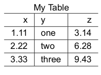
Figure 16.9: A kable table
The kable function takes a data frame as input and a number of formatting parameters,
returning a formatted table suitable for display.
kable produces great-looking output, but many people discover they want more control over the output than it allows.
Luckily kable can be paired with another package, kableExtra, for—not surprisingly—extra kable functionality.
Here we set the rounding and caption using kable.
Then we use kable_styling to make the table more narrow than full width,
add shaded striping in our LaTeX output,
and center the table on our output.
library(knitr)
library(kableExtra)

kable(myTable, digits = 2, caption = 'My Table') %>%
   kable_styling(full_width = FALSE,
                 latex_options = c('hold_position', 'striped'),
                 position = "center",
                 font_size = 12)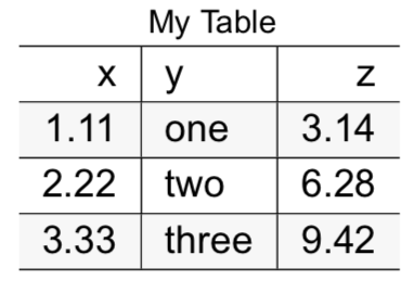
Figure 16.10: A kableExtra table
The kable_styling function takes a kable table as input (not a data frame) plus
formatting parameters, then returns a formatted table.
Some options in kable_styling have a different impact on your output depending on your output format.
In our previous example, the full_width = FALSE does not change anything in LaTeX (PDF) format
because tables in LaTeX output default to not being full width.
In HTML, however, the default behavior for kable tables is to be full width, so this option has an impact.
Similiarly, the latex_options = c('hold_position', 'striped') option applies only to LaTeX output, not HTML.
The 'hold_position' ensures that the table ends up where we put it in our source, not at the top or bottom of the page,
which tends to happen in LaTeX.
The 'striped' option makes zebra-striped tables with alternating light and dark rows for easier reading.
For more control over Microsoft Word tables, we recommend the function flextable::regulartable,
which is discussed in Recipe 16.14, “Generating Microsoft Word Output”.
16.11 Inserting Math Equations
Problem
You want to insert a mathematical equation in your document.
Solution
R Markdown supports the LaTeX math equation notation. There are two ways of entering LaTeX in R Markdown.
For short formulas, put the LaTeX notation inline between single dollar signs.
The volume of a sphere, for example, could be expressed as $\beta = (X^{T}X)^{-1}X^{T}{\bf{y}}$,
which would result in this inline formula \(\beta = (X^{T}X)^{-1}X^{T}{\bf{y}}\).
For large formula blocks, embed the block between double dollar signs, like this block:
$$
\frac{\partial \mathrm C}{ \partial \mathrm t } + \frac{1}{2}\sigma^{2}
      \mathrm S^{2} \frac{\partial^{2} \mathrm C}{\partial \mathrm C^2}
    + \mathrm r \mathrm S \frac{\partial \mathrm C}{\partial \mathrm S}\ =
    \mathrm r \mathrm C
    \label{eq:1}
$$
which generates this output:
\[ \frac{\partial \mathrm C}{ \partial \mathrm t } + \frac{1}{2}\sigma^{2} \mathrm S^{2} \frac{\partial^{2} \mathrm C} {\partial \mathrm C^2} + \mathrm r \mathrm S \frac{\partial \mathrm C} {\partial \mathrm S}\ = \mathrm r \mathrm C \label{eq:1} \]
Discussion
The math equation markup syntax is a LaTeX standard that originated in TeX. Building on that standard, R Markdown can render mathematical expressions in PDF, HTML, MS Word, and MS PowerPoint documents. The PDF and HTML formats support a full range of LaTeX math equations. The translation into Microsoft Word and PowerPoint, however, supports only a subset of the full syntax.
The details of LaTeX equation notation are beyond the scope of this book, but since TeX has been around for 40+ years there are many great resources available online and in many books. A very good online resource is the Wikibooks.org introduction to LaTeX/Mathematics.
16.12 Generating HTML Output
Problem
You would like to create a HyperText Markup Language (HTML) document from an R Markdown document.
Solution
In RStudio, click on the arrow next to the button labeled Knit at the top of the code editing window. When you do, you’ll get a drop-down list of all the output formats available for your current document. Select the option for Knit to HTML, as shown in Figure 16.11.
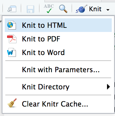
Figure 16.11: Knit to HTML
Discussion
When you click Knit to HTML, RStudio moves html_document: default to the top of your YAML output chunk at the top of the document, saves the file, and then runs rmarkdown::render('./*YourFile*.Rmd'). If you have knitted your document into three different formats, your YAML may look like this:
output:
  html_document: default
  pdf_document: default
  word_document: default
If you run render('./*YourFile*.Rmd') on your R Markdown document, substituting your actual filename for *YourFile*.Rmd, it will, by default, knit to the topmost output format (in this case, HTML).
If you are knitting to HTML, your R Markdown document should not contain any special LaTeX-specific formatting, as these will not knit properly in HTML. The exception, as mentioned in prior recipes, is LaTeX math equations, which show up properly in HTML, thanks to the MathJax JavaScript library.
See Also
Recipe 16.11, “Inserting Math Equations”
16.13 Generating PDF Output
Problem
You would like to create an Adobe Portable Document Format (PDF) document from an R Markdown document.
Solution
In RStudio, click on the arrow next to the button labeled Knit at the top of the code editing window. When you do, you’ll get a drop-down list of all the output formats available for your current document. Select the option for Knit to PDF, as shown in Figure 16.12.
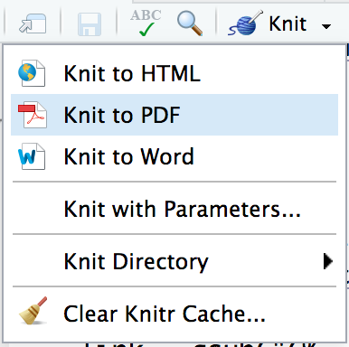
Figure 16.12: Knit to PDF
This will move pdf_document to the top of your YAML output options:
---
title: "Nice Title"
output:
  pdf_document: default
  html_document: default
---
and then knit the document to PDF.
Discussion
Knitting to PDF uses Pandoc and a LaTeX engine to generate a PDF document. If you don’t already have a LaTeX distribution installed on your computer, the easiest way to get one is with the tinytex package. Install tinytex in R, then call install_tinytex(), and tinytex will install a small and efficient LaTeX distribution on your computer:
LaTeX is rich with options and, fortunately, most things that we want to do can be represented with R Markdown and automatically converted to LaTeX via Pandoc. Since LaTeX is a powerful typesetting tool, it is possible to do things with it for which there is no R Markdown equivalent. We can’t enumerate all possibilities here, but we can talk about the ways to pass parameters directly to LaTeX from R Markdown. Keep in mind, though, that any LaTeX-specific options you use will not be translated properly into other formats, like HTML or MS Word.
There are two main ways to pass information from R Markdown to the LaTeX rendering engine:
- Pass LaTeX directly to the LaTeX compiler.
- Set LaTeX options in the YAML header.
If we want to pass LaTeX commands directly through to the LaTeX compiler, we can use the LaTeX command beginning with \. The limitation is that if you knit the document to any format other than PDF, the command following the slash is completely omitted from the output.
For example, if we put this phrase into our R Markdown source:
Sometimes you want to write directly in \LaTeX !
it will be rendered as:

Figure 16.13: LaTeX typeset
However, if you render your document to HTML the \LaTeX command will be dropped completely leaving you with an unappealing blank in your document.
If we want to set global options for LaTeX, you can do so by adding parameters to the YAML header in our R Markdown document. The YAML header has top-level metadata as well as subdata for some options. Different parameters are set at different levels of indentation, so we typically look them up in R Markdown: The Definitive Guide just to be sure.
For example, if you have some previously written LaTeX content and you want to include it in your document, you can add this prewritten content in three different places in your document: in the header, before the body content, or after the body content at the end. If you were adding external content in all three sections, your YAML header would look like this:
---
title: "My Wonderful Document"
output:
  pdf_document:
    includes:
      in_header: header_stuff.tex
      before_body: body_prefix.tex
      after_body: body_suffix.tex
---
Another common LaTex option to use is a LaTeX template for formatting your document. Many templates are available online, and some companies and schools have their own templates. If you want to use an existing template, you can reference it in the YAML header like this:
---
title: "Poetry I Love"
output:
  pdf_document:
    template: i_love_template.tex
---
And you can also turn on or off page numbering and section numbering:
---
title: "Why I Love a Good ToC"
output:
  pdf_document:
    toc: true
    number_sections: true
---
Some LaTeX options, however, get set with top-level YAML metadata:
---
title: "Custom Report"
output: pdf_document
fontsize: 12pt
geometry: margin=1.2in
---
So when you are setting LaTeX options, consult the R Markdown documentation to determine if the option you are setting is a suboption of the output: parameter or its own top-level YAML option.
See Also
The section “PDF document” from R Markdown: The Definitive Guide
16.14 Generating Microsoft Word Output
Problem
You would like to create a Microsoft Word document from an R Markdown document.
Solution
In RStudio, click on the arrow next to the button labeled Knit at the top of the code editing window. When you do, you’ll get a drop-down list of all the output formats available for your current document. Select the option for Knit to Word, as shown in Figure 16.14.
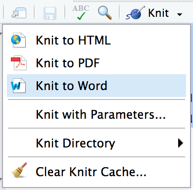
Figure 16.14: Knit to Word
This will move word_document to the top of your YAML output options and then knit your R Markdown document:
---
title: "Nice Title"
output:
  word_document: default
  pdf_document: default
---
Discussion
Knitting to Microsoft Word is helpful in businesses and scholastic environments where supervisors and collaborators expect documents in Word format. Most R Markdown features work very well in Word, but there are a few tweaks we have found to be helpful when using Word output.
Microsoft has its own equation editing tool. Pandoc will coerce your LaTeX equations into MS Equation Editor, which works well with most basic equations but does not support all LaTeX equation options. One challenge is that MS Equation Editor does not support changing fonts for part of an equation. As a result, matrix notation with fractions and other formulas that require varying fonts can look a bit odd in Word.
Here’s a matrix example that looks good in HTML and PDF:
$$
M = \begin{bmatrix}
       \frac{1}{6} & \frac{1}{6} & 0           \\[0.3em]
       \frac{7}{8} & 0           & \frac{2}{3} \\[0.3em]
       0           & \frac{7}{9} & \frac{7}{7}
     \end{bmatrix}
$$
which renders as this in HTML and PDF: \[ M = \begin{bmatrix} \frac{1}{6} & \frac{1}{6} & 0 \\[0.3em] \frac{7}{8} & 0 & \frac{2}{3} \\[0.3em] 0 & \frac{7}{9} & \frac{7}{7} \end{bmatrix} \] But looks like Figure 16.15 in MS Word.
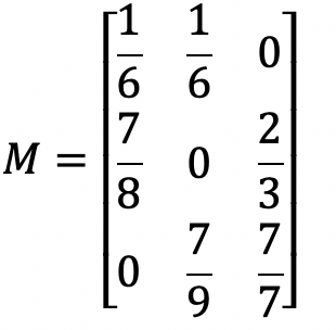
Figure 16.15: Matrix in MS Word
Any formula using scaling of characters will not work properly in Word. For example:
$( \big( \Big( \bigg( \Bigg($would look like this in HTML and LaTex:
\(( \big( \Big( \bigg( \Bigg(\)
but will get simplified in MS Equation Editor, as shown in Figure 16.16.
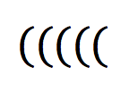
Figure 16.16: Equation font scaling in MS Word
The easiest solution for equations in Word is to try your equation first. If you don’t like the output, take your LaTeX equation to an online free equation editor, and render your equation there, and save it as an image file. Then include that image file in your R Markdown document, ensuring that your Word documents have rendered equations that look as good as HTML or LaTeX documents. You will probably want to save your LaTeX equation source in a text file just to make sure you can alter it easily later.
Another challenge with Word output is that often figures don’t look quite as good as they do in HTML or PDF. Take this example of a line graph:
```{r}
mtcars %>%
  group_by(cyl, gear) %>%
  summarize(mean_hp=mean(hp)) %>%
  ggplot(., aes(x = cyl, y = mean_hp, group = gear)) +
    geom_point() +
    geom_line(aes(linetype = factor(gear))) +
    theme_bw()
```
In a Word document this image appears as Figure 16.17.
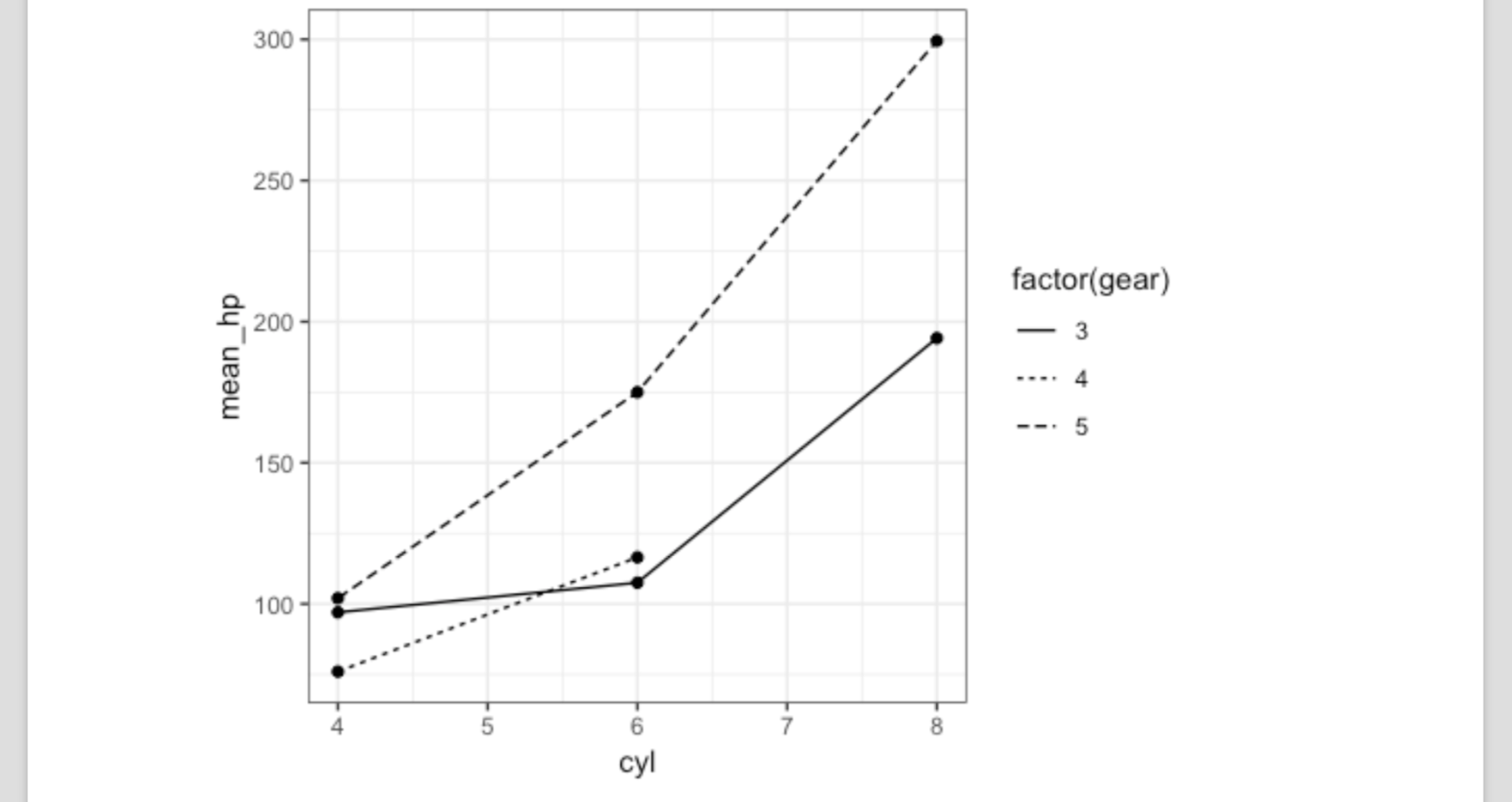
Figure 16.17: Graph in Word
This looks pretty good, but when printed, the image looks a little blocky and not sharp.
You can improve this by increasing the dots per inch (dpi) setting used when knitting the output. This will help make the output smoother and sharper:
```{r, dpi=300}
mtcars %>%
  group_by(cyl, gear) %>%
  summarize(mean_hp=mean(hp)) %>%
  ggplot(., aes(x = cyl, y = mean_hp, group = gear)) +
    geom_point() +
    geom_line(aes(linetype = factor(gear))) +
    theme_bw()
```
To show the improvement in appearance, we’ve stitched together a composite image showing the default low dpi on the left and the higher dpi on the right in Figure 16.18.
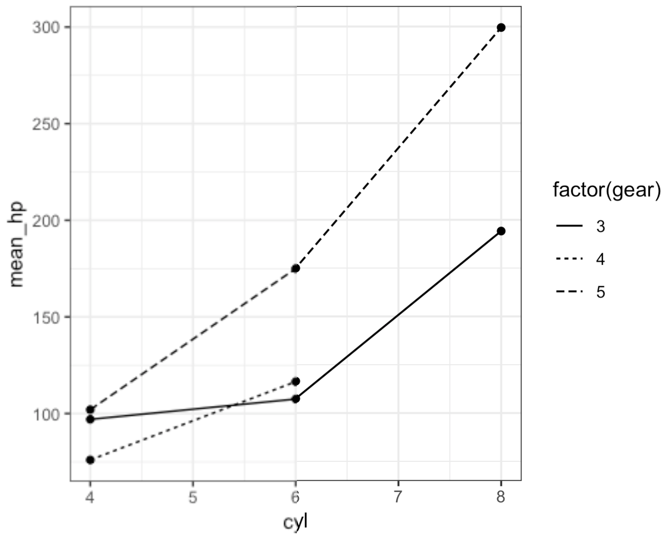
Figure 16.18: Image resolution in Word
In addition to images, table output in Word sometimes is not as customized as we desire. Using kable, as illustrated in previous recipes, produces a good, no-frills table in MS Word:
library(knitr)
myTable <- tibble(x = c(1.111, 2.222, 3.333),
                 y = c('one', 'two', 'three'),
                 z = c(5, 6, 7))
kable(myTable, caption = 'My Table in Word') | x | y | z |
|---|---|---|
| 1.11 | one | 5 |
| 2.22 | two | 6 |
| 3.33 | three | 7 |
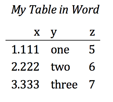
Figure 16.19: Table in Word
which renders like Figure 16.19 in MS Word.
Pandoc puts the table in a MS table structure inside the Word document.
But, just like with tables in PDFs or HTML, we can use the flextable package in Word too.
which gives us Figure 16.20 in Word:
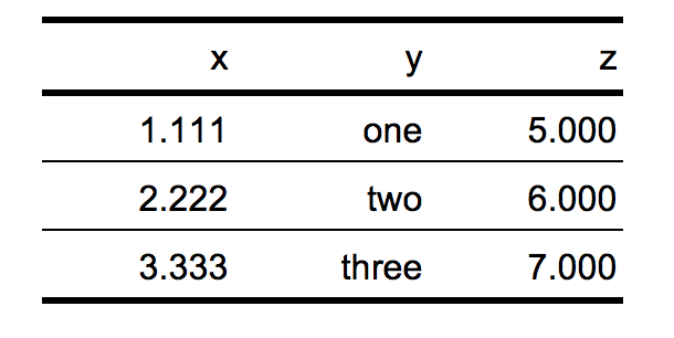
Figure 16.20: regulartable in Word
We can tap into to the rich formatting features of flextable and pipe chains to adjust the column widths,
add background color to our headers, and make the header font white:
regulartable(myTable) %>%
   width(width = c(.5, 1.5, 3)) %>%
   bg(bg = "#000080", part = "header") %>%
   color(color = "white", part = "header")
which gives us Figure 16.21 in Word.
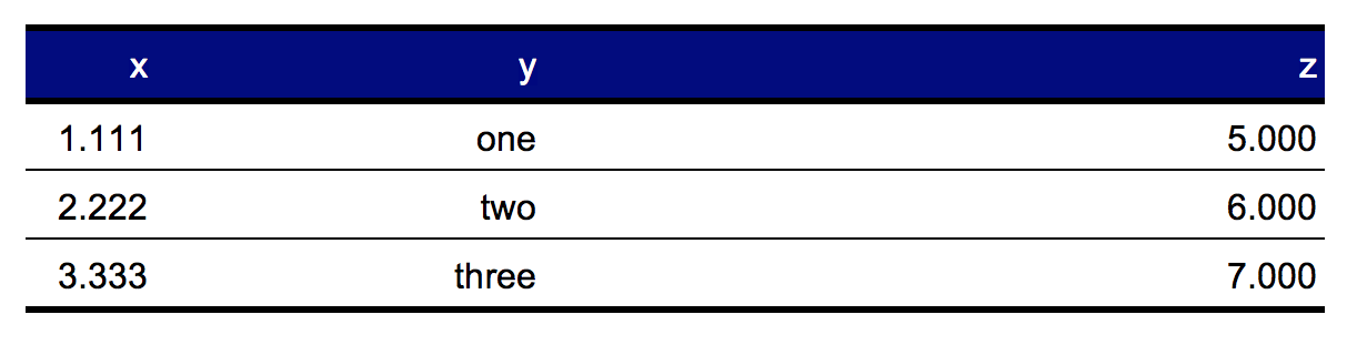
Figure 16.21: A customized regulartable in Word
For details on all the customizable options in flextable, see the flextable vignettes and the flextable online documentation.
Knitting to Word allows a template to control the formatting of your Word output.
To use a template, add reference_docs: your_template.docx to the YAML header:
---
title: "Nice Title"
output:
  word_document:
     reference_docx: template.docx
---
When you knit an R Markdown file to Word using a template, knitr maps the formatting of elements in your source document to styles in the template. So if you want to change the font of the body text, then you would set the body text style in a Word template to your desired font. Then knitr will use the template style in the new document.
A common workflow when using a template for the first time is to knit your document to Word without a template. Then open the resulting Word document, adjust the styles of each section to your preference, and use the adjusted Word document as a template in the future. This way, you don’t have to guess what style knitr is using for each element.
See Also
The flextable vignette on formatting: vignette('format','flextable' )
flextable online documentation.
16.15 Generating Presentation Output
Problem
You would like to create a presentation from an R Markdown document.
Solution
R Markdown and knitr support creating presentations from R Markdown documents. The most common formats for presentations are HTML (using ioslides or Slidy HTML templates), PDF with Beamer, or Microsoft PowerPoint. The biggest difference between R Markdown documents and R Markdown presentations is that presentations default to landscape layout (wide, not long), and every time you create a second-level header starting with ##, knitr will create a new “page” or slide.
The easiest way to get started with presentations with R Markdown is to use RStudio and select: File -> New File -> R Markdown… Then choose one of the four presentation formats offered by the dialog in Figure 16.22.
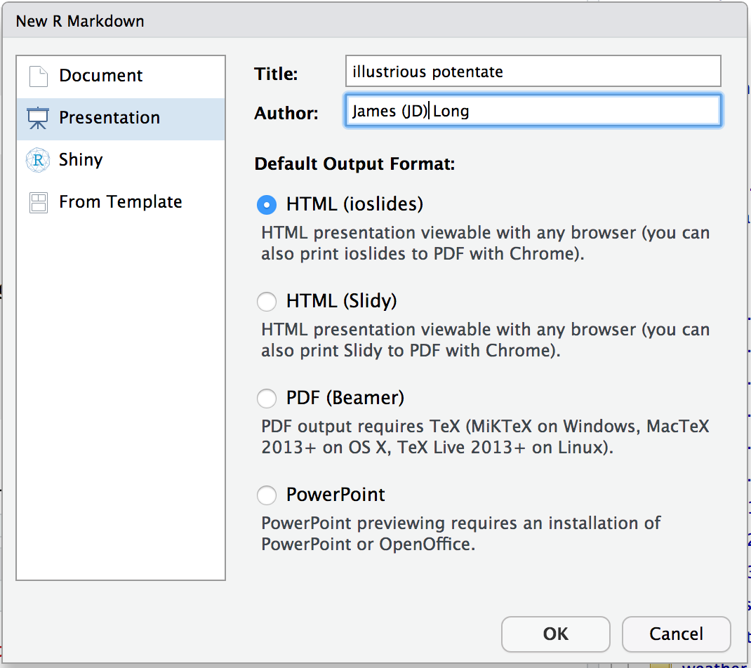
Figure 16.22: New R Markdown document: Presentations
The four classes of presentations map to the three major classes of documents discussed in previous document recipes.
When it comes time to knit your document to an output format, in RStudio you can select the drop-down list from the Knit button and select the type of presentation you would like to produce, as shown in Figure 16.23.
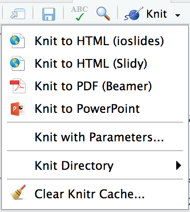
Figure 16.23: Knit: Presentations
Discussion
Knitting to a presentation format is very similar to knitting to a regular document, only with different output names. When you use the Knit button in RStudio to choose your output format, RStudio moves your selected output format to the top of the output options in the YAML header of your document, then runs rmarkdown::render("*your_file*.Rmd"), which knits to the topmost format in your YAML header.
For example, if we selected Knit to PDF (Beamer), the header of the presentation might look like this:
---
title: "Best Presentation Ever"
output:
  beamer_presentation: default
  slidy_presentation: default
  ioslides_presentation: default
  powerpoint_presentation: default
---
Most of the HTML options discussed in previous HTML recipes apply to Slidy and ioslides HTML presentations. Beamer is a PDF-based format, so most LaTex and PDF options discussed in previous recipes apply to Beamer. And last, but never least, PowerPoint is a Microsoft format, so the caveats and options discussed previously about Word documents apply to PowerPoint as well.
See Also
The other recipes related to R Markdown output can be helpful: Recipes 16.12, “Generating HTML Output”, 16.13, “Generating PDF Output”, and 16.14, “Generating Microsoft Word Output”.
16.16 Creating a Parameterized Report
Problem
You would like to run the same report periodically with different inputs.
Solution
R Markdown documents can be created with parameters in the YAML header that can then be used as variables in the document body. The parameters are stored as named items in a list called params, which you can access in your code chunk.
Later, if we want to change the parameter(s), we have three options:
- Edit the R Markdown document and then render it again.
- Render the document from within R using the command
rmarkdown::render, passing parameters as a list.
- Using RStudio, select the Knitr menu, then Knit with Parameters, and RStudio will prompt you for parameters before knitting.
Discussion
Using parameters in R Markdown is very helpful if you have a document you need to run regularly with different settings. A common use case is a report in which only a date setting and a label are changed each time it runs.
Here’s an example R Markdown document illustrating how parameters can be passed into the text of a document:
---
title: "Example of Params"
output: html_document
params:
  effective_date: '2018-07-01'
  quarter_num: 2
---

## Illustrate Params
```{r, results='asis', echo=FALSE}
cat('### Quarter', params$quarter_num,
    'report. Valuation date:',
    params$effective_date)
```
The rendered R Markdown results in Figure 16.24.
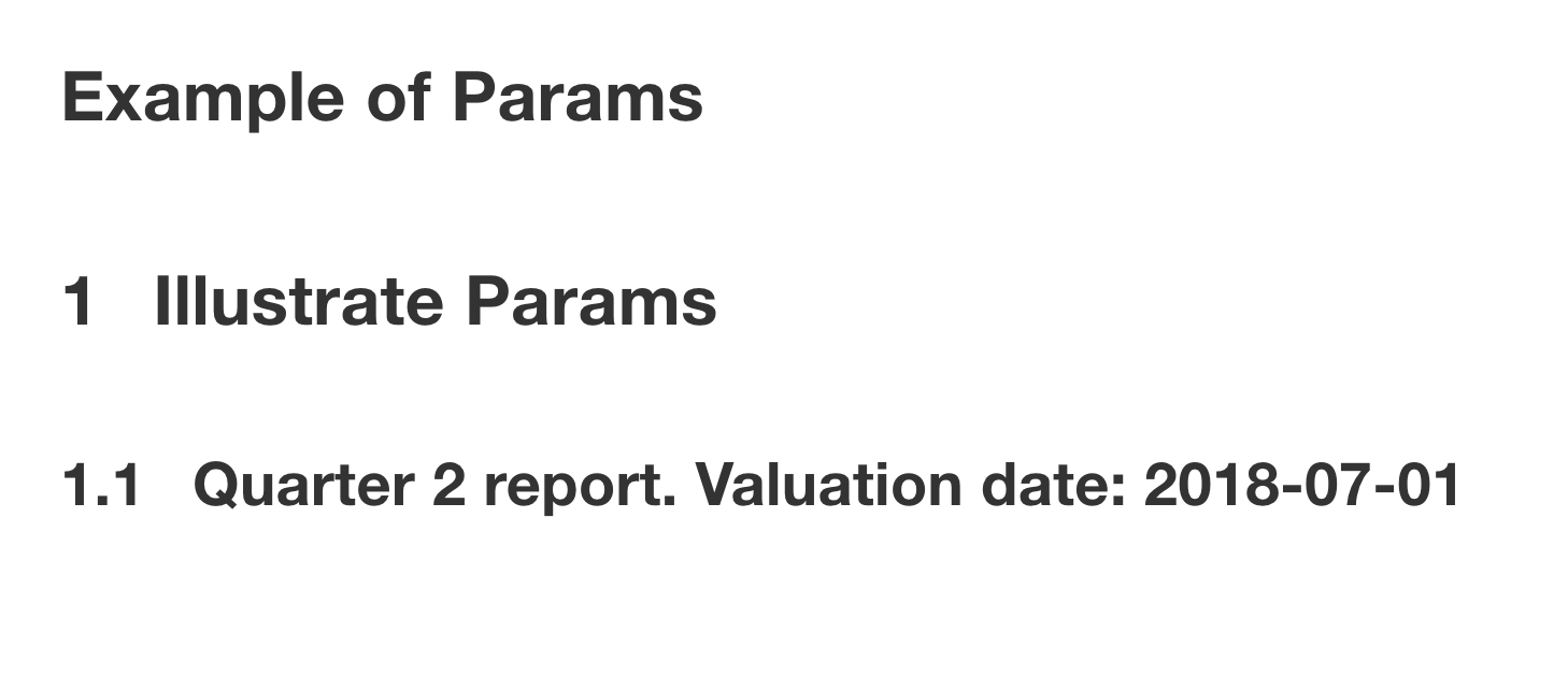
Figure 16.24: Parameter output
In the header of the chunk, we set results='asis',
because our code chunk is going to generate Markdown text directly.
We want to dump that Markdown into our document
without prefixing it with ##, which is what normally happens to the output from a code chunk.
In addition, inside the code block we use cat to concatenate our text together.
We use cat here instead of paste because cat performs less conversion on the text than calling paste.
This ensures that the text is simply put together and passed into the Markdown document without being altered.
If we want to render the document with other parameters, we can edit the default values in the YAML header and then knit. Or we can use the Knitr menu (Figure 16.25) to knit with parameters.
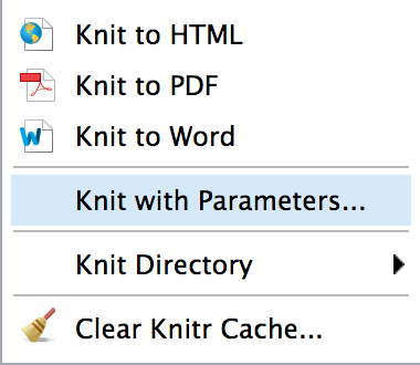
Figure 16.25: Knit with Parameters from Knitr menu
This then prompts us for parameters, as shown in Figure 16.26.
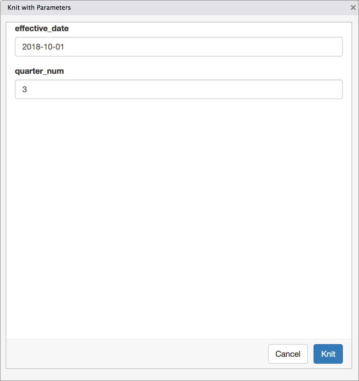
Figure 16.26: Knit with Parameters
Or we can render the document from R, passing new parameters as a list:
rmarkdown::render("example_of_params.Rmd",
                  params = list(quarter_num=2,
                                effective_date='2018-07-01'))
As an alternative to using the Knitr menu, if we want to be prompted for parameters we can set params="ask" when we call rmarkdown::render and R will prompt us for inputs.
See Also
See the RStudio online documentation on parameterized reports.
16.17 Organizing Your R Markdown Workflow
Problem
You want to organize your R Markdown project so that it’s efficient, flexible, and productive.
Solution
The best way to get control of your project is to organize your workflow. Organization takes a bit of effort, so it might be overkill to have a highly structured project if your R Markdown document is only one page of output with three small code chunks. However, most people find that organizing their workflow is worth the added effort.
Here are four tips for organizing your workflow so that your work is easier to read, edit, and maintain in the future:
- Use RStudio Projects
- Directory Naming
- Create an R Package for Reused Logic
- R Markdown Should Focus on Content, Logic Should be Sourced
Use RStudio Projects
RStudio includes the notion of an RStudio Project (note the capital P), which is a way of storing metadata and settings related to a logical project. When you open a Project in RStudio, one of the things that RStudio does is set the working directory to the path where the Project is located. Every Project should live in its own unique directory. All code is run from that working directory, which means your code should never contain setwd commands that would keep your analysis from being run on someone else’s computer.
Name directories intuitively
Inside your Project directory it’s a good idea to organize your files into directories and then name your files thoughtfully inside those directories. As the number of files in a project increases, so does the importance of organization and intuitive naming. One common structure recommended by the team at Software Carpentry is this:
my_project
 |- data
 |- doc
 |- results
 |- src
In this structure, raw input data goes in the data directory, documentation goes in doc, results of analysis go in results, and R source code goes in src.
Once you have a directory structure to put your work into, the individual files should be named in a way that’s readable to both humans and computers. This helps with maintaining your code in the future and saves a lot of headaches. Some of the best advice we’ve seen on file naming comes from Jenny Bryan:
- Use underscores instead of spaces in filenames; spaces cause too many headaches later.
- If you put dates in your filenames, use ISO 8601 dates: YYYY-MM-DD.
- Use a prefix on your scripts so they sort properly—for example, 00_start_here.R, 01_data_scrub.R, 02_report_output.Rmd.
Using numeric prefixes on your scripts and using ISO 8601 dates helps ensure that your files sort in a meaningful way by default. This is very helpful when someone else, or even future you, tries to make sense of your project.
Create an R package for reused logic
Once you have a good directory structure and rational naming, you should give some thought as to what logic goes where. You should consider building an R package for logic you use in more than three different projects. R packages are collections of functions and other code that provide functionality not available in Base R. Throughout this book we’ve used a number of packages, and there’s nothing stopping you from writing a package for your functions that you use over and over. Building a package is out of scope for this book, but one of the best introductions to the topic is Jim Hester’s presentation “You Can Make a Package in 20 Minutes”.
Keep R Markdown focused on content, and source logic
Most of us start a project with one big .Rmd file full of all our logic in code chunks. As the document grows and the code chunks expand, this can get difficult to manage. You may find that your code formatting is intermingled with code that reshapes data and fetches things from files and databases. Having logic, formatting, and presentation code all intermingled can make it hard to alter your code later and even harder for someone else to understand your code. We recommend keeping the code blocks in your main reporting .Rmd file focused on content, tables, and figures and having your manipulation logic stored in _*.R_ files that you pull in with the source function.
Using source to pull in external R code involves passing the filename of your R file to the source function:
R will run the entire contents of *my_logic_file*.R at the place in your code where you call source. A good pattern is to source files that extract data frames and reshape your data into the form you need to make graphs or tables in your document. Then, in your main R Markdown, you keep mostly code that prepares graphs and tables.
Keep in mind that this is a design pattern for managing large, unwieldy R Markdown files. If your project is not very large, you should probably just keep all your code in the .Rmd file.
See Also
Project-Oriented Workflow tidyverse documentation
Project Management with RStudio from Software Carpentry
R Packages by Hadley Wickham (O’Reilly)
Naming Things by Jenny Bryan
Good Enough Practices in Scientific Computing by Greg Wilson, et al.