3 Navigating the Software

Introduction

Both R and RStudio are big chunks of software, first and foremost. You will inevitably spend time doing what one does with any big piece of software: configuring it, customizing it, updating it, and fitting it into your computing environment. This chapter will help you perform those tasks. There is nothing here about numerics, statistics, or graphics. This is all about dealing with R and RStudio as software.

3.1 Getting and Setting the Working Directory

Problem

You want to change your working directory, or you just want to know what it is.

Solution

RStudio: Navigate to a directory in the Files pane. Then from the Files pane, select More → Set As Working Directory, as shown in Figure 3.1.

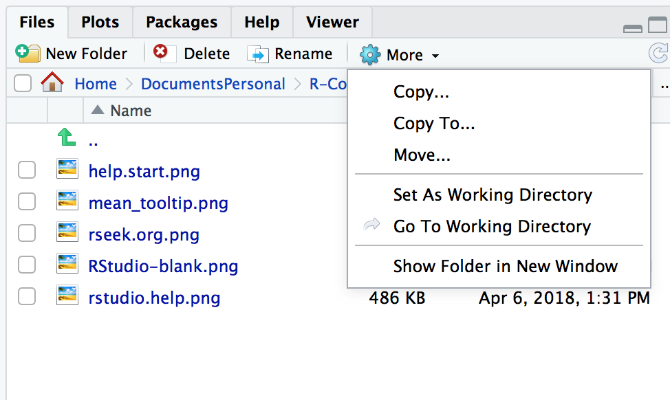
Figure 3.1: RStudio: Set As Working Directory

Console: Use getwd to report the working directory, and use setwd to change it:

getwd()
#> [1] "/home/travis/build/CerebralMastication/R-Cookbook"

setwd("~/Documents/MyDirectory")

Discussion

Your working directory is important because it is the default location for all file input and output—including reading and writing data files, opening and saving script files, and saving your workspace image. When you open a file and do not specify an absolute path, R will assume that the file is in your working directory.

If you’re using RStudio projects, your default working directory will be the home directory of the project. See Recipe 3.2, “Creating a New R Studio Project”, for more about creating RStudio projects.

3.2 Creating a New RStudio Project

Problem

You want to create a new RStudio project to keep all your files related to a specific project.

Solution

Click File → New Project as in Figure 3.2

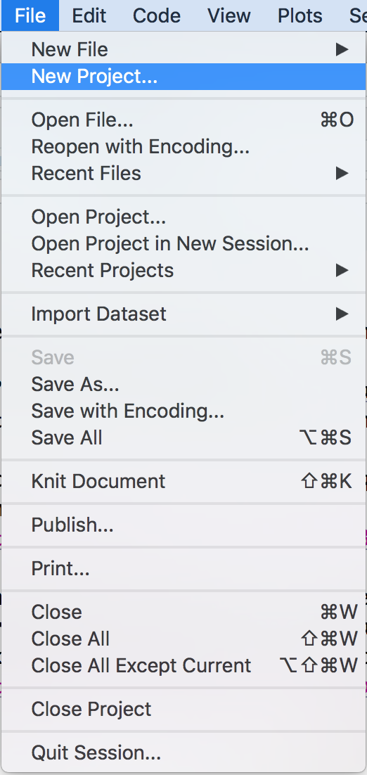
Figure 3.2: Selecting New Project

This will open the New Project dialog box and allow you to choose which type of project you would like to create, as shown in Figure 3.3.

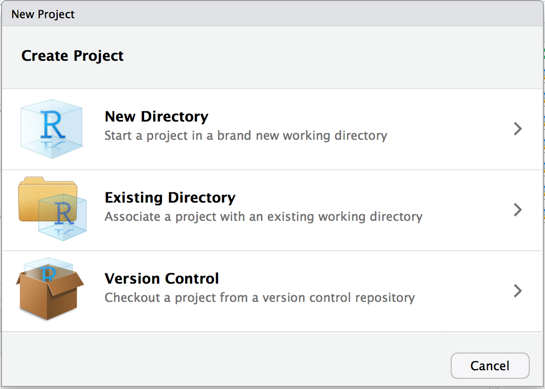
Figure 3.3: New Project dialog

Discussion

Projects are a powerful concept that’s specific to RStudio. They help you by doing the following:

Setting your working directory to the project directory.
Preserving window state in RStudio so when you return to a project your windows are all as you left them. This includes opening any files you had open when you last saved your project.
Preserving RStudio project settings.

To hold your project settings, RStudio creates a project file with an .Rproj extension in the project directory. If you open the project file in RStudio, it works like a shortcut for opening the project. In addition, RStudio creates a hidden directory named .Rproj.user to house temporary files related to your project.

Any time you’re working on something nontrivial in R we recommend creating an RStudio project. Projects help you stay organized and make your project workflow easier.

3.3 Saving Your Workspace

Problem

You want to save your workspace and all variables and functions you have in memory.

Solution

Call the save.image function:

save.image()

Discussion

Your workspace holds your R variables and functions, and it is created when R starts. The workspace is held in your computer’s main memory and lasts until you exit from R. You can easily view the contents of your workspace in RStudio in the Environment tab, as shown in Figure 3.4

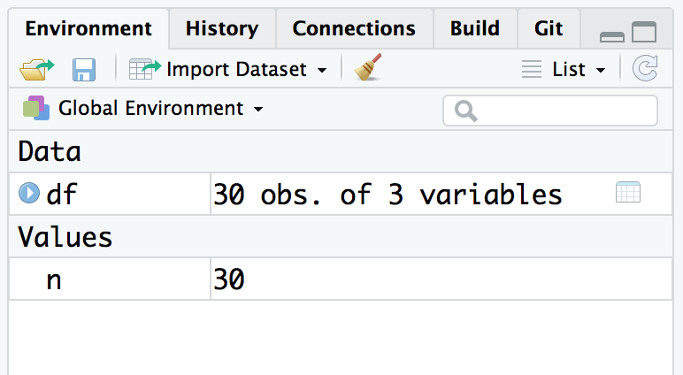
Figure 3.4: RStudio environment

However, you may want to save your workspace without exiting R, because you know bad things mysteriously happen when you close your laptop to carry it home. In this case, use the save.image function.

The workspace is written to a file called .RData in the working directory. When R starts, it looks for that file and, if it finds it, initializes the workspace from it.

Sadly, the workspace does not include your open graphs: for example, that cool graph on your screen disappears when you exit R. The workspace also does not include the position of your windows or your RStudio settings. This is why we recommend using RStudio projects and writing your R scripts so that you can reproduce everything you’ve created.

3.4 Viewing Your Command History

Problem

You want to see your recent sequence of commands.

Solution

Depending on what you are trying to accomplish, you can use a few different methods to access your prior command history. If you are in the RStudio console pane, you can press the up arrow to interactively scroll through past commands.

If you want to see a listing of past commands, you can either execute the history function or access the History pane in RStudio to view your most recent input:

history()

In RStudio typing history() into the console simply activates the History pane in RStudio (Figure 3.5). You could also make that pane visible by clicking on it with your cursor.

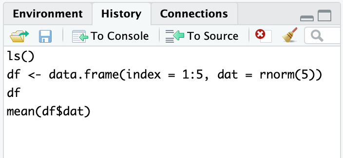
Figure 3.5: RStudio History pane

Discussion

The history function displays your most recent commands. In RStudio the history command will activate the History pane. If you were running R outside of RStudio, history shows the most recent 25 lines, but you can request more like so:

history(100)          # Show 100 most recent lines of history
history(Inf)          # Show entire saved history

From within RStudio, the History tab shows an exhaustive list of past commands in chronological order, with the most recent at the bottom of the list. You can highlight past commands with your cursor, then click on “To Console” or “To Source” to copy past commands into the console or source editor, respectively. This can be terribly handy when you’ve done interactive data analysis and then decide you want to save some past steps to a source file for later use.

From the console you can see your history by simply pressing the up arrow to scroll backward through your input, which causes your previous typing to reappear, one line at a time.

If you’ve exited from R or RStudio, you can still see your command history. R saves the history in a file called .Rhistory in the working directory. Open the file with a text editor and then scroll to the bottom; you will see your most recent typing.

3.5 Saving the Result of the Previous Command

Problem

You typed an expression into R that calculated the value, but you forgot to save the result in a variable.

Solution

A special variable called .Last.value saves the value of the most recently evaluated expression. Save it to a variable before you type anything else.

Discussion

It is frustrating to type a long expression or call a long-running function but then forget to save the result. Fortunately, you needn’t retype the expression nor invoke the function again—the result was saved in the .Last.value variable:

aVeryLongRunningFunction()  # Oops! Forgot to save the result!
x <- .Last.value            # Capture the result now

A word of caution here: the contents of .Last.value are overwritten every time you type another expression, so capture the value immediately. If you don’t remember until another expression has been evaluated, it’s too late!

3.6 Displaying Loaded Packages via the Search Path

Problem

You want to see the list of packages currently loaded into R.

Solution

Use the search function with no arguments:

search()

Discussion

The search path is a list of packages that are currently loaded into memory and available for use. Although many packages may be installed on your computer, only a few of them are actually loaded into the R interpreter at any given moment. You might be wondering which packages are loaded right now.

With no arguments, the search function returns the list of loaded packages. It produces an output like this:

search()
#>  [1] ".GlobalEnv"        "package:knitr"     "package:forcats"  
#>  [4] "package:stringr"   "package:dplyr"     "package:purrr"    
#>  [7] "package:readr"     "package:tidyr"     "package:tibble"   
#> [10] "package:ggplot2"   "package:tidyverse" "package:stats"    
#> [13] "package:graphics"  "package:grDevices" "package:utils"    
#> [16] "package:datasets"  "package:methods"   "Autoloads"        
#> [19] "package:base"

Your machine may return a different result, depending on what’s installed there. The return value of search is a vector of strings. The first string is ".GlobalEnv", which refers to your workspace. Most strings have the form "package:*packagename*", which indicates that the package called *packagename* is currently loaded into R. In the preceding example, you can see many tidyverse packages installed, including purrr, ggplot2, and tibble.

R uses the search path to find functions. When you type a function name, R searches the path—in the order shown—until it finds the function in a loaded package. If the function is found, R executes it. Otherwise, it prints an error message and stops. (There is actually a bit more to it: the search path can contain environments, not just packages, and the search algorithm is different when initiated by an object within a package; see the R Language Definition for details.)

Since your workspace (.GlobalEnv) is first in the list, R looks for functions in your workspace before searching any packages. If your workspace and a package both contain a function with the same name, your workspace will “mask” the function; this means that R stops searching after it finds your function and so never sees the package function. This is a blessing if you want to override the package function…and a curse if you still want access to it. If you find yourself feeling cursed because you (or some package you loaded) overrode a function (or other object) from an existing loaded package, you can use the full *environment*::*name* form to call an object from a loaded package environment. For example, if you wanted to call the dplyr function count, you could do so using dplyr::count. Using the full explicit name to call a function will work even if you have not loaded the package. So if you have dplyr installed but not loaded, you can still call dplyr::count. It is becoming increasingly common with online examples to show the full *packagename*::*function* in examples. While this removes ambiguity about where a function comes from, it makes example code very wordy.

Note that R will include only loaded packages in the search path. So if you have installed a package, but not loaded it by using library(*packagename*), then R will not add that package to the search path.

R also uses the search path to find R datasets (not files) or any other object via a similar procedure.

Unix and Mac users: don’t confuse the R search path with the Unix search path (the PATH environment variable). They are conceptually similar but two distinct things. The R search path is internal to R and is used by R only to locate functions and datasets, whereas the Unix search path is used by the OS to locate executable programs.

3.7 Viewing the List of Installed Packages

Problem

You want to know what packages are installed on your machine.

Solution

Use the library function with no arguments for a basic list. Use installed.packages to see more detailed information about the packages.

Discussion

The library function with no arguments prints a list of installed packages. The list can be quite long.

library()

In RStudio, the list is displayed in a new tab in the editor window.

You can get more details via the installed.packages function, which returns a matrix of information regarding the packages on your machine. Each row corresponds to one installed package. The columns contain information such as package name, library path, and version. The information is taken from R’s internal database of installed packages.

To extract useful information from this matrix, use normal indexing methods. The following snippet calls installed.packages and extracts both the Package and Version columns for the first five packages, letting you see what version of each package is installed:

installed.packages()[1:5, c("Package", "Version")]
#>            Package      Version
#> abind      "abind"      "1.4-5"
#> askpass    "askpass"    "1.1"  
#> assertthat "assertthat" "0.2.1"
#> backports  "backports"  "1.1.4"
#> base64enc  "base64enc"  "0.1-3"

3.8 Accessing the Functions in a Package

Problem

A package installed on your computer is either a standard package or a package you’ve downloaded. When you try using functions in the package, however, R cannot find them.

Solution

Use either the library function or the require function to load the package into R:

library(packagename)

Discussion

R comes with several standard packages, but not all of them are automatically loaded when you start R. Likewise, you can download and install many useful packages from CRAN or GitHub, but they are not automatically loaded when you run R. The MASS package comes standard with R, for example, but you could get this message when using the lda function in that package:

lda(x)
#> Error in lda(x): could not find function "lda"

R is complaining that it cannot find the lda function among the packages currently loaded into memory.

When you use the library function or the require function, R loads the package into memory and its contents become immediately available to you:

my_model <- 
  lda(cty ~ displ + year, data = mpg)
#> Error in lda(cty ~ displ + year, data = mpg): could not find function "lda"

library(MASS)                          # Load the MASS library into memory
#> 
#> Attaching package: 'MASS'
#> The following object is masked from 'package:dplyr':
#> 
#>     select
my_model <-
  lda(cty ~ displ + year, data = mpg)  # Now R can find the function

Before you call library, R does not recognize the function name. Afterward, the package contents are available and calling the lda function works.

Notice that you needn’t enclose the package name in quotes.

The require function is nearly identical to library. It has two features that are useful for writing scripts. It returns TRUE if the package was successfully loaded and FALSE otherwise. It also generates a mere warning if the load fails—unlike library, which generates an error.

Both functions have a key feature: they do not reload packages that are already loaded, so calling twice for the same package is harmless. This is especially nice for writing scripts. The script can load needed packages while knowing that loaded packages will not be reloaded.

The detach function will unload a package that is currently loaded:

detach(package:MASS)

Observe that the package name must be qualified, as in package:MASS.

One reason to unload a package is that it contains a function whose name conflicts with a same-named function lower on the search list. When such a conflict occurs, we say the higher function masks the lower function. You no longer “see” the lower function because R stops searching when it finds the higher function. Hence, unloading the higher package unmasks the lower name.

3.9 Accessing Built-in Datasets

Problem

You want to use one of R’s built-in datasets, or you want to access one of the datasets that comes with another package.

Solution

The standard datasets distributed with R are already available to you, since the datasets package is in your search path. If you’ve loaded any other packages, datasets that come with those loaded packages will also be available in your search path.

To access datasets in other packages, use the data function while giving the dataset name and package name:

data(dsname, package = "pkgname")

Discussion

R comes with many built-in datasets. Other packages, such as dplyr and ggplot2, also come with example data that’s used in the examples found in their help files. These datasets are useful when you are learning about R, since they provide data with which to experiment.

Many datasets are kept in a package called (naturally enough) datasets, which is distributed with R. That package is in your search path, so you have instant access to its contents. For example, you can use the built-in dataset called pressure:

head(pressure)
#>   temperature pressure
#> 1           0   0.0002
#> 2          20   0.0012
#> 3          40   0.0060
#> 4          60   0.0300
#> 5          80   0.0900
#> 6         100   0.2700

If you want to know more about pressure, use the help function to learn about it and other datasets:

help(pressure)      # Bring up help page for pressure dataset

You can see a table of contents for datasets by calling the data function with no arguments:

data()              # Bring up a list of datasets

Any R package can elect to include datasets that supplement those supplied in datasets. The MASS package, for example, includes many interesting datasets. Use the data function to load a dataset from a specific package by using the package argument. MASS includes a dataset called Cars93, which you can load into memory in this way:

data(Cars93, package = "MASS")

After this call to data, the Cars93 dataset is available to you; then you can execute summary(Cars93), head(Cars93), and so forth.

When attaching a package to your search list (e.g., via library(MASS)), you don’t need to call data. Its datasets become available automatically when you attach it.

You can see a list of available datasets in MASS, or any other package, by using the data function with a package argument and no dataset name:

data(package = "pkgname")

3.10 Installing Packages from CRAN

Problem

You found a package on CRAN, and now you want to install it on your computer.

Solution

R code: Use the install.packages function, putting the name of the package in quotes:

install.packages("packagename")

RStudio: The Packages window in RStudio helps make installing new R packages straightforward. All packages that are installed on your machine are listed in the Packages window, along with description and version information. To load a new package from CRAN, click on the Install button near the top of the Packages window, as shown in Figure 3.6.

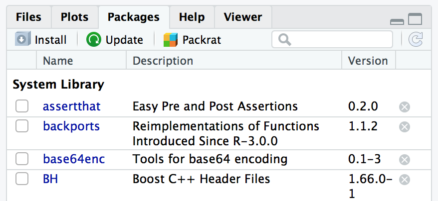
Figure 3.6: RStudio Packages window

Discussion

Installing a package locally is the first step toward using it. If you are installing packages outside of RStudio, the installer may prompt you for a mirror site from which it can download the package files. It will then display a list of CRAN mirror sites. The top CRAN mirror is 0-Cloud. This is typically the best option, as it connects you to a globally mirrored content delivery network (CDN) sponsored by RStudio. If you want to select a different mirror, choose one geographically close to you.

The official CRAN server is a relatively modest machine generously hosted by the Department of Statistics and Mathematics at WU Wien, Vienna, Austria. If every R user downloaded from the official server, it would buckle under the load, so there are numerous mirror sites around the globe. In RStudio the default CRAN server is set to be the RStudio CRAN mirror. The RStudio CRAN mirror is accessible to all R users, not just those running the RStudio IDE.

If the new package depends upon other packages that are not already installed locally, then the R installer will automatically download and install those required packages. This is a huge benefit that frees you from the tedious task of identifying and resolving those dependencies.

There is a special consideration when you are installing on Linux or Unix. You can install the package either in the systemwide library or in your personal library. Packages in the systemwide library are available to everyone; packages in your personal library are (normally) used only by you. So a popular, well-tested package would likely go in the systemwide library, whereas an obscure or untested package would go into your personal library.

By default, install.packages assumes you are performing a systemwide install. If you do not have sufficient user permissions to install in the systemwide library location, R will ask if you would like to install the package in a user library. The default that R suggests is typically a good choice. However, if you would like to control the path for your library location, you can use the lib= argument of the install.packages function:

install.packages("packagename", lib = "~/lib/R")

Or you can change your default CRAN server as described in Recipe 3.12, “Setting or Changing a Default CRAN Mirror”.

3.11 Installing a Package from GitHub

Problem

You’ve found an interesting package you’d like to try. However, the author has not yet published the package on CRAN, but has published it on GitHub. You’d like to install the package directly from GitHub.

Solution

Ensure you have the devtools package installed and loaded:

install.packages("devtools")
library(devtools)

Then use install_github and the name of the GitHub repository to install directly from GitHub. For example, to install Thomas Lin Pederson’s tidygraph package, you would execute the following:

install_github("thomasp85/tidygraph")

Discussion

The devtools package contains helper functions for installing R packages from remote repositories, like GitHub. If a package has been built as an R package and then hosted on GitHub, you can install the package using the install_github function by passing the GitHub username and repository name as a string parameter. You can determine the GitHub username and repo name from the GitHub URL, or from the top of the GitHub page, as in the example shown in Figure 3.7.

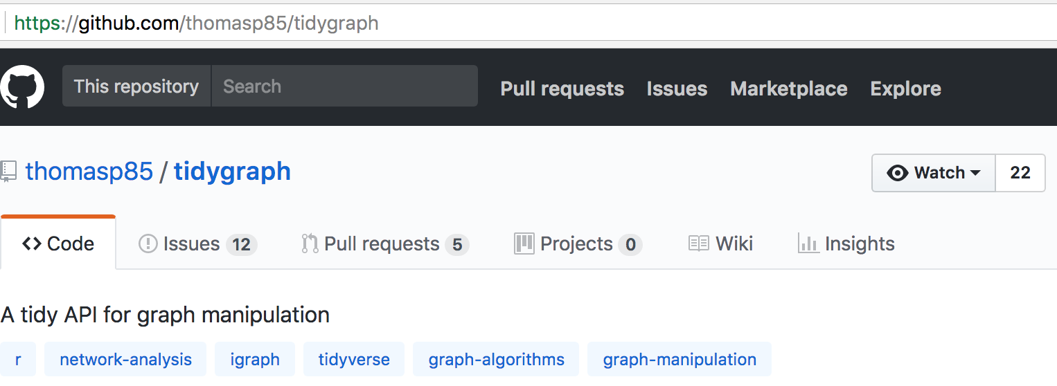
Figure 3.7: Example GitHub project page

3.12 Setting or Changing a Default CRAN Mirror

Problem

You are downloading packages. You want to set or change your default CRAN mirror.

Solution

In RStudio, you can change your default CRAN mirror from the RStudio Preferences menu shown in Figure 3.8.

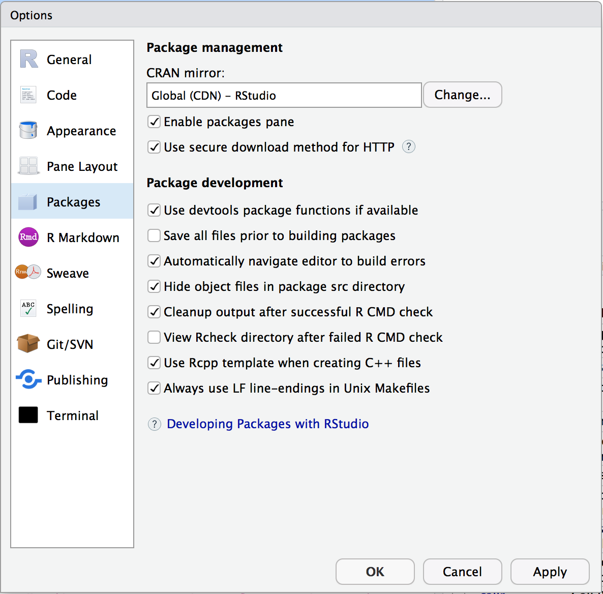
Figure 3.8: RStudio package preferences

If you are running R without RStudio, you can change your CRAN mirror using the following solution. This solution assumes you have an .Rprofile, as described in Recipe 3.16, “Customizing R Startup”:

Call the chooseCRANmirror function:

chooseCRANmirror()

R will present a list of CRAN mirrors.

Select a CRAN mirror from the list and press OK.
To get the URL of the mirror, look at the first element of the repos option:

options("repos")[[1]][1]

Add this line to your .Rprofile file. If you want the RStudio CRAN mirror, you would do the following:

options(repos = c(CRAN = "http://cran.rstudio.com"))

Or you could use the URL of another CRAN mirror.

Discussion

When you install packages, you probably use the same CRAN mirror each time (namely, the mirror closest to you or the RStudio mirror) because RStudio does not prompt you every time you load a package; it simply uses the setting from the Preferences menu. You may want to change that mirror to use a different mirror that’s closer to you or controlled by your employer. Use this solution to change your repo so that every time you start R or RStudio, you will be using your desired repo.

The repos option is the name of your default mirror. The chooseCRANmirror function has the important side effect of setting the repos option according to your selection. The problem is that R forgets the setting when it exits, leaving no permanent default. By setting repos in your .Rprofile, you restore the setting every time R starts.

3.13 Running a Script

Problem

You captured a series of R commands in a text file. Now you want to execute them.

Solution

The source function instructs R to read the text file and execute its contents:

source("myScript.R")

Discussion

When you have a long or frequently used piece of R code, capture it inside a text file. That lets you easily rerun the code without having to retype it. Use the source function to read and execute the code, just as if you had typed it into the R console.

Suppose the file hello.R contains this one, familiar greeting:

print("Hello, World!")

Then sourcing the file will execute the file contents:

source("hello.R")
#> [1] "Hello, World!"

Setting echo=TRUE will echo the script lines before they are executed, with the R prompt shown before each line:

source("hello.R", echo = TRUE)
#> 
#> > print("Hello, World!")
#> [1] "Hello, World!"

3.14 Running a Batch Script

Problem

You are writing a command script, such as a shell script in Unix or macOS or a BAT script in Windows. Inside your script, you want to execute an R script.

Solution

Run the R program with the CMD BATCH subcommand, giving the script name and the output file name:

R CMD BATCH scriptfile outputfile

If you want the output sent to stdout or if you need to pass command-line arguments to the script, consider the Rscript command instead:

Rscript scriptfile arg1 arg2 arg3

Discussion

R is normally an interactive program, one that prompts the user for input and then displays the results. Sometimes you want to run R in batch mode, reading commands from a script. This is especially useful inside shell scripts, such as scripts that include a statistical analysis.

The CMD BATCH subcommand puts R into batch mode, reading from *scriptfile* and writing to *outputfile*. It does not interact with a user.

You will likely use command-line options to adjust R’s batch behavior to your circumstances. For example, using --quiet silences the startup messages that would otherwise clutter the output:

R CMD BATCH --quiet myScript.R results.out

Other useful options in batch mode include the following:

--slave: Like --quiet, but it makes R even more silent by inhibiting echo of the input.
--no-restore: At startup, do not restore the R workspace. This is important if your script expects R to begin with an empty workspace.
--no-save: At exit, do not save the R workspace. Otherwise, R will save its workspace and overwrite the .RData file in the working directory.
--no-init-file: Do not read either the *.Rprofile* or *~/.Rprofile* file.

The CMD BATCH subcommand normally calls proc.time when your script completes, showing the execution time. If this annoys you, then end your script by calling the q function with runLast=FALSE, which will prevent the call to proc.time.

The CMD BATCH subcommand has two limitations: the output always goes to a file, and you cannot easily pass command-line arguments to your script. If either limitation is a problem, consider using the Rscript program that comes with R. The first command-line argument is the script name, and the remaining arguments are given to the script:

Rscript myScript.R arg1 arg2 arg3

Inside the script, you can access the command-line arguments by calling commandArgs, which returns the arguments as a vector of strings:

argv <- commandArgs(TRUE)

The Rscript program takes the same command-line options as CMD BATCH, which were just described.

Output is written to stdout, which R inherits from the calling shell script, of course. You can redirect the output to a file by using the normal redirection:

Rscript --slave myScript.R arg1 arg2 arg3 >results.out

Here is a small R script, arith.R, that takes two command-line arguments and performs four arithmetic operations on them:

argv <- commandArgs(TRUE)
x <- as.numeric(argv[1])
y <- as.numeric(argv[2])

cat("x =", x, "\n")
cat("y =", y, "\n")
cat("x + y = ", x + y, "\n")
cat("x - y = ", x - y, "\n")
cat("x * y = ", x * y, "\n")
cat("x / y = ", x / y, "\n")

The script is invoked like this:

Rscript arith.R 2 3.1415

which produces the following output:

x = 2
y = 3.1415
x + y = 5.1415
x - y = -1.1415
x * y = 6.283
x / y = 0.6366385

On Linux, Unix, or Mac, you can make the script fully self-contained by placing a #! line at the head with the path to the Rscript program. Suppose that Rscript is installed in /usr/bin/Rscript on your system. Adding this line to arith.R makes it a self-contained script:

#!/usr/bin/Rscript --slave

argv <- commandArgs(TRUE)
x <- as.numeric(argv[1])
.
. (etc.)
.

At the shell prompt, we mark the script as executable:

chmod +x arith.R

Now we can invoke the script directly without the Rscript prefix:

arith.R 2 3.1415

3.15 Locating the R Home Directory

Problem

You need to know the R home directory, which is where the configuration and installation files are kept.

Solution

R creates an environment variable called R_HOME that you can access by using the Sys.getenv function:

Sys.getenv("R_HOME")
#> [1] "/home/travis/R-bin/lib/R"

Discussion

Most users will never need to know the R home directory. But system administrators or sophisticated users must know it in order to check or change the R installation files.

When R starts, it defines a system environment variable (not an R variable) called R_HOME, which is the path to the R home directory. The Sys.getenv function can retrieve the systerm environment variable value. Here are examples by platform. The exact value reported will almost certainly be different on your own computer:

On Windows

> Sys.getenv("R_HOME")
[1] "C:/PROGRA~1/R/R-34~1.4"

On macOS

> Sys.getenv("R_HOME")
[1] "/Library/Frameworks/R.framework/Resources"

On Linux or Unix

> Sys.getenv("R_HOME")
[1] "/usr/lib/R"

The Windows result looks funky because R reports the old, DOS-style compressed pathname. The full, user-friendly path would be C:\Program Files\R\R-3.4.4 in this case.

On Unix and macOS, you can also run the R program from the shell and use the RHOME subcommand to display the home directory:

R RHOME
# /usr/lib/R

Note that the R home directory on Unix and macOS contains the installation files but not necessarily the R executable file. The executable could be in /usr/bin while the R home directory is, for example, /usr/lib/R.

3.16 Customizing R Startup

Problem

You want to customize your R sessions by, for instance, changing configuration options or preloading packages.

Solution

Create a script called .Rprofile that customizes your R session. R will execute the .Rprofile script when it starts. The placement of .Rprofile depends upon your platform:

macOS, Linux, or Unix: Save the file in your home directory (~/.Rprofile).
Windows: Save the file in your Documents directory.

Discussion

R executes profile scripts when it starts allowing you to tweak the R configuration options.

You can create a profile script called .Rprofile and place it in your home directory (macOS, Linux, Unix) or your Documents directory (Windows). The script can call functions to customize your sessions, such as this simple script that sets two environment variables and sets the console prompt to R>:

Sys.setenv(DB_USERID = "my_id")
Sys.setenv(DB_PASSWORD = "My_Password!")
options(prompt = "R> ")

The profile script executes in a bare-bones environment, so there are limits on what it can do. Trying to open a graphics window will fail, for example, because the graphics package is not yet loaded. Also, you should not attempt long-running computations.

You can customize a particular project by putting an .Rprofile file in the directory that contains the project files. When R starts in that directory, it reads the local .Rprofile file; this allows you to do project-specific customizations (e.g., setting your console prompt to a specific project name). However, if R finds a local profile, then it does not read the global profile. That can be annoying, but it’s easily fixed: simply source the global profile from the local profile. On Unix, for instance, this local profile would execute the global profile first and then execute its local material:

source("~/.Rprofile")
#
# ... remainder of local .Rprofile...
#

Setting Options

Some customizations are handled via calls to the options function, which sets the R configuration options. There are many such options, and the R help page for options lists them all:

help(options)

Here are some examples:

browser="*path*": Path of default HTML browser
digits=n: Suggested number of digits to print when printing numeric values
editor="*path*": Default text editor
prompt="*string*": Input prompt
repos="*url*": URL for default repository for packages
warn=n: Controls display of warning messages

Reproducibility

Many of us use certain packages over and over in all of our scripts. For example, we use the tidyverse packages in almost all our scripts. It is tempting to load these packages in your .Rprofile so that they are always available without you typing anything. As a matter of fact, this advice was given in the first edition of this book. However, the downside of loading packages in your .Rprofile is reproducibility. If someone else (or you, on another machine) tries to run your script, they may not realize that you had loaded packages in your .Rprofile. Your script might not work for them, depending on which packages they load. So while it might be convenient to load packages in .Rprofile, you will play better with collaborators (and your future self) if you explicitly call library(*packagename*) in your R scripts.

Another issue with reproducibility and the .Rprofile is when users change calculation default behaviors of R inside their .Rprofile. An example of this would be setting options(stringsAsFactors = FALSE). This is appealing, as many users would prefer this default. However, if someone runs the script without this option being set, they will get different results or not be able to run the script at all. This can lead to considerable frustration.

As a guideline, you should primarly put things in the .Rprofile that:

Change the look and feel of R (e.g., digits)
Are specific to your local environment (e.g., browser)
Specifically need to be outside of your scripts (i.e., database passwords)
Do not change the results of your analysis

Startup Sequence

Here is a simplified overview of what happens when R starts (type **help(Startup)** to see the full details):

R executes the Rprofile.site script. This is the site-level script that enables system administrators to override default options with localizations. The script’s full path is R_HOME/etc/Rprofile.site. (R_HOME is the R home directory; see Recipe 3.15, “Locating the R Home Directory”.)

The R distribution does not include an Rprofile.site file. Rather, the system administrator creates one if it is needed.
R executes the .Rprofile script in the working directory; or, if that file does not exist, executes the .Rprofile script in your home directory. This is the user’s opportunity to customize R for his or her purposes. The .Rprofile script in the home directory is used for global customizations. The .Rprofile script in a lower-level directory can perform specific customizations when R is started there—for instance, customizing R when started in a project-specific directory.
R loads the workspace saved in .RData, if that file exists in the working directory. R saves your workspace in the file called .RData when it exits. It reloads your workspace from that file, restoring access to your local variables and functions. You can disable this behavior in RStudio through Tools → Global Options. We recommend you disable this option and always explicitly save and load your work.
R executes the .First function, if you defined one. The .First function is a useful place for users or projects to define startup initialization code. You can define it in your .Rprofile or in your workspace.
R executes the .First.sys function. This step loads the default packages. The function is internal to R and not normally changed by either users or administrators.

Note that R does not load the default packages until the final step, when it executes the .First.sys function. Before that, only the base package has been loaded. This is a key point, because it means the previous steps cannot assume that packages other than the base are available. It also explains why trying to open a graphics window in your .Rprofile script fails: the graphics packages aren’t loaded yet.

3.17 Using R and RStudio in the Cloud

Problem

You want to run R and RStudio in a cloud environment.

Solution

The most straightforward way to use R in the cloud is to use the RStudio.cloud web service. To use the service, point your web browser to http://rstudio.cloud and set up an account, or log in with your Google or GitHub credentials.

Discussion

After you log in, click New Project to begin a new RStudio session in a new workspace. You’ll be greeted by the familiar RStudio interface shown in Figure 3.9.

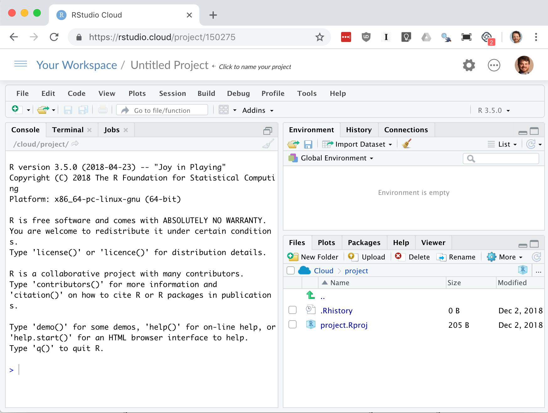
Figure 3.9: RStudio.cloud

Keep in mind that as of this writing the RStudio.cloud service is in alpha testing and may not be 100% stable. Your work will persist after you log off. However, as with any system, it is a good idea to ensure you have backups of all the work you do. A common work pattern is to connect your project in RStudio.cloud to a GitHub.com repository and push your changes frequently from Rstudio.cloud to GitHub. This workflow has been used significantly in the writing of this book.

Use of git and GitHub are beyond the scope of this book, but if you are interested in learning more, we highly recommend Jenny Bryan’s web book Happy Git and GitHub for the useR.

In its current alpha state, RStudio.cloud limits each session to 1 GB of RAM and 3 GB of drive space. So it’s a great platform for learning and teaching but might not (yet) be the platform on which you want to build a commercial data science laboratory. RStudio has expressed its intent to offer greater processing power and storage as part of a paid tier of service as the platform matures.

If you need more computing power than offered by RStudio.cloud and you are willing to pay for the services, both Amazon AWS and Google Cloud Platform offer cloud-based RStudio offerings. Other cloud platforms that support Docker, such as Digital Ocean, are also reasonable options for cloud-hosted RStudio.

3 Navigating the Software

Introduction

3.1 Getting and Setting the Working Directory

Problem

Solution

Discussion

See Also

3.2 Creating a New RStudio Project

Problem

Solution

Discussion

3.3 Saving Your Workspace

Problem

Solution

Discussion

See Also

3.4 Viewing Your Command History

Problem

Solution

Discussion

3.5 Saving the Result of the Previous Command

Problem

Solution

Discussion

See Also

3.6 Displaying Loaded Packages via the Search Path

Problem

Solution

Discussion

See Also

3.7 Viewing the List of Installed Packages

Problem

Solution

Discussion

See Also

3.8 Accessing the Functions in a Package

Problem

Solution

Discussion

See Also

3.9 Accessing Built-in Datasets

Problem

Solution

Discussion

See Also

3.10 Installing Packages from CRAN

Problem

Solution

Discussion

See Also

3.11 Installing a Package from GitHub

Problem

Solution

Discussion

3.12 Setting or Changing a Default CRAN Mirror

Problem

Solution

Discussion

See Also

3.13 Running a Script

Problem

Solution

Discussion

See Also

3.14 Running a Batch Script

Problem

Solution

Discussion

See Also

3.15 Locating the R Home Directory

Problem

Solution

Discussion

On Windows

On macOS

On Linux or Unix

3.16 Customizing R Startup

Problem

Solution

Discussion