13 Beyond Basic Numerics and Statistics
Introduction
This chapter presents a few advanced techniques such as those you might encounter in the first or second year of a graduate program in applied statistics.
Most of these recipes use functions available in the base distribution. Through add-on packages, R provides some of the world’s most advanced statistical techniques. This is because researchers in statistics now use R as their lingua franca, showcasing their newest work. Anyone looking for a cutting-edge statistical technique is urged to search CRAN and the web for possible implementations.
13.1 Minimizing or Maximizing a Single-Parameter Function
Problem
Given a single-parameter function f, you want to find the point at
which f reaches its minimum or maximum.
Solution
To minimize a single-parameter function, use optimize. Specify the
function to be minimized and the bounds for its domain (x):
If you instead want to maximize the function, specify maximum = TRUE:
Discussion
The optimize function can handle functions of one argument. It
requires upper and lower bounds for x that delimit the region to be
searched. The following example finds the minimum of a polynomial,
3x4 – 2x3 + 3x2 – 4x + 5:
f <- function(x)
  3 * x ^ 4 - 2 * x ^ 3 + 3 * x ^ 2 - 4 * x + 5
optimize(f, lower = -20, upper = 20)
#> $minimum
#> [1] 0.597
#>
#> $objective
#> [1] 3.64
The returned value is a list with two elements: minimum, the x value
that minimizes the function; and objective, the value of the function
at that point.
A tighter range for lower and upper means a smaller region to be
searched and hence a faster optimization. However, if you are unsure of
the appropriate bounds, then use big but reasonable values such as
lower = -1000 and upper = 1000. Just be careful that your function does
not have multiple minima within that range! The optimize function will
find and return only one such minimum.
See Also
See Recipe 13.2, “Minimizing or Maximizing a Multiparameter Function”.
13.2 Minimizing or Maximizing a Multiparameter Function
Problem
Given a multiparameter function f, you want to find the point at which
f reaches its minimum or maximum.
Solution
To minimize a multiparameter function, use optim. You must specify the
starting point, which is a vector of initial arguments for f:
To maximize the function instead, specify this control parameter:
Discussion
The optim function is more general than optimize
(see Recipe 13.1, “Minimizing or Maximizing a Single-Parameter Function”)
because it handles multiparameter functions. To evaluate your function
at a point, optim packs the point’s coordinates into a vector and
calls your function with that vector. The function should return a
scalar value. optim will begin at your starting point and move through
the parameter space, searching for the function’s minimum.
Here is an example of using optim to fit a nonlinear model. Suppose
you believe that the paired observations z and x are related by
zi = (xi + α)β + εi, where α and β are
unknown parameters and where the εi are nonnormal noise terms.
Let’s fit the model by minimizing a robust metric, the sum of the
absolute deviations:
∑|z – (x + a)b|
First we define the function to be minimized. Note that the function has only one formal parameter, a two-element vector. The actual parameters to be evaluated, a and b, are packed into the vector in locations 1 and 2:
load(file = './data/opt.rdata')  # loads x, y, z

f <-
  function(v) {
    a <- v[1]
    b <- v[2]                           # "Unpack" v, giving a and b
    sum(abs(z - ((x + a) ^ b)))         # calculate and returns the error
  }
The following code makes a call to optim, starts from (1, 1), and searches for the minimum
point of f:
optim(c(1, 1), f)
#> $par
#> [1] 10.0  0.7
#>
#> $value
#> [1] 1.26
#>
#> $counts
#> function gradient
#>      485       NA
#>
#> $convergence
#> [1] 0
#>
#> $message
#> NULL
The returned list includes convergence, the indicator of success or
failure. If this indicator is 0, then optim found a minimum; otherwise,
it did not. Obviously, the convergence indicator is the most important
returned value because other values are meaningless if the algorithm did
not converge.
The returned list also includes par, the parameters that minimize our
function, and value, the value of f at that point. In this case,
optim did converge and found a minimum point at approximately a =
10.0 and b = 0.7.
There are no lower and upper bounds for optim, just the starting point
that you provide. A better guess for the starting point means a faster
minimization.
The optim function supports several different minimization algorithms,
and you can select among them. If the default algorithm does not work
for you, see the help page for alternatives. A typical problem with
multidimensional minimization is that the algorithm gets stuck at a
local minimum and fails to find a deeper, global minimum. Generally
speaking, the algorithms that are more powerful are less likely to get
stuck. However, there is a trade-off: they also tend to run more slowly.
See Also
The R community has implemented many tools for optimization. On CRAN, see the task view for Optimization and Mathematical Programming for more solutions.
13.3 Calculating Eigenvalues and Eigenvectors
Problem
You want to calculate the eigenvalues or eigenvectors of a matrix.
Solution
Use the eigen function. It returns a list with two elements, values
and vectors, which contain (respectively) the eigenvalues and
eigenvectors.
Discussion
Suppose we have a matrix such as the Fibonacci matrix:
Given the matrix, the eigen function will return a list of its
eigenvalues and eigenvectors:
eigen(fibmat)
#> eigen() decomposition
#> $values
#> [1]  1.618 -0.618
#>
#> $vectors
#>       [,1]   [,2]
#> [1,] 0.526 -0.851
#> [2,] 0.851  0.526
Use either eigen(fibmat)$values or eigen(fibmat)$vectors to select
the needed value from the list.
13.4 Performing Principal Component Analysis
Problem
You want to identify the principal components of a multivariable dataset.
Solution
Use the prcomp function. The first argument is a formula whose
righthand side is the set of variables, separated by plus signs (+).
The lefthand side is empty:
Discussion
The base software for R includes two functions for principal component
analysis (PCA), prcomp and princomp. The documentation mentions that
prcomp has better numerical properties, so that’s the function
presented here.
An important use of PCA is to reduce the dimensionality of your dataset. Suppose your data contains a large number N of variables. Ideally, all the variables are more or less independent and contributing equally. But if you suspect that some variables are redundant, the PCA can tell you the number of sources of variance in your data. If that number is near N, then all the variables are useful. If the number is less than N, then your data can be reduced to a dataset of smaller dimensionality.
The PCA recasts your data into a vector space where the first dimension
captures the most variance, the second dimension captures the second
most, and so forth. The actual output from prcomp is an object that,
when printed, gives the needed vector rotation:
load(file = './data/pca.rdata')
r <- prcomp(~ x + y)
print(r)
#> Standard deviations (1, .., p=2):
#> [1] 0.393 0.163
#>
#> Rotation (n x k) = (2 x 2):
#>      PC1    PC2
#> x -0.553  0.833
#> y -0.833 -0.553
We typically find the summary of PCA much more useful. It shows the proportion of variance that is captured by each component:
summary(r)
#> Importance of components:
#>                          PC1   PC2
#> Standard deviation     0.393 0.163
#> Proportion of Variance 0.853 0.147
#> Cumulative Proportion  0.853 1.000
In this example, the first component captured 85% of the variance and the second component only 15%, so we know the first component captured most of it.
After calling prcomp, use plot(r) to view a bar chart of the
variances of the principal components and predict(r) to rotate your
data to the principal components.
See Also
See Recipe 13.9, “Factor Analysis” for an example of using principal component analysis. Further uses of PCA in R are discussed in Modern Applied Statistics with S-Plus by W. N. Venables and B. D. Ripley (Springer).
13.5 Performing Simple Orthogonal Regression
Problem
You want to create a linear model using orthogonal regression in which the variances of x and y are treated symmetrically.
Solution
Use prcomp to perform PCA on x and y.
From the resulting rotation, compute the slope and intercept:
Discussion
Orthogonal regression is also known as total least squares (TLS).
The ordinary least squares (OLS) algorithm has an odd property: it is
asymmetric. That is, calculating lm(y ~ x) is not the mathematical inverse of calculating lm(x ~ y).
The reason is that OLS assumes the x values to be constants and the
y values to be random variables, so all the variance is attributed to
y and none is attributed to x. This creates an asymmetric situation.
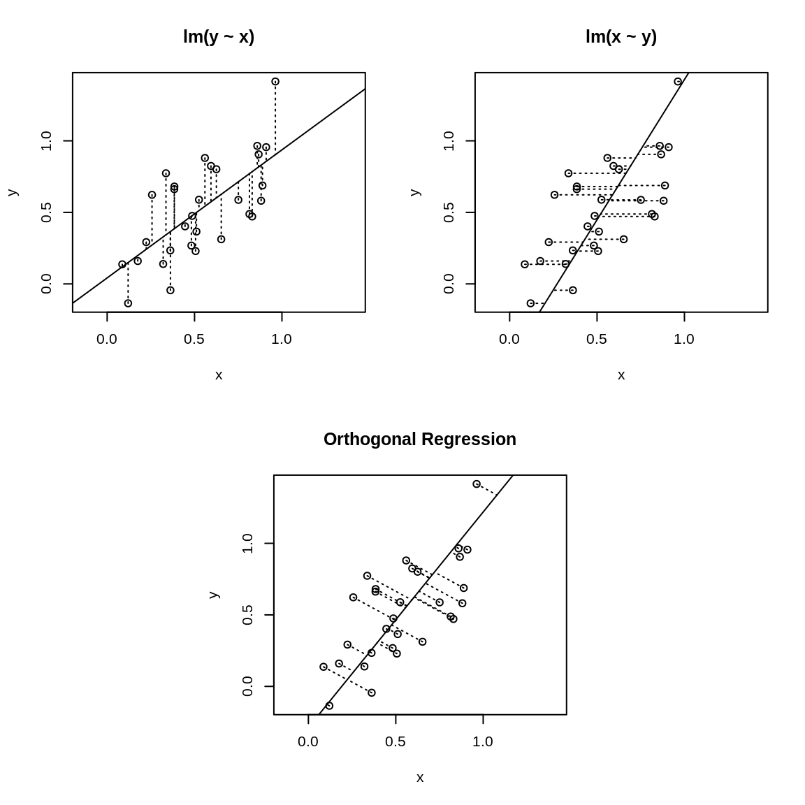
Figure 13.1: Ordinary least squares versus orthogonal regression
The asymmetry is illustrated in Figure 13.1 where the upper-left
panel displays the fit for lm(y ~ x). The OLS algorithm tries the minimize the vertical
distances, which are shown as dotted lines. The upper-right panel shows
the identical dataset but fit with lm(x ~ y) instead, so the algorithm is minimizing the horizontal
dotted lines. Obviously, you’ll get a different result depending upon
which distances are minimized.
The lower panel of Figure 13.1 is quite different. It uses PCA to implement orthogonal regression. Now the distances being minimized are the orthogonal distances from the data points to the regression line. This is a symmetric situation: reversing the roles of x and y does not change the distances to be minimized.
Implementing a basic orthogonal regression in R is quite simple. First, perform the PCA:
Next, use the rotations to compute the slope:
and then, from the slope, calculate the intercept:
We call this a “basic” regression because it yields only the point estimates for the slope and intercept, not the confidence intervals. Obviously, we’d like to have the regression statistics, too. Recipe 13.8, “Bootstrapping a Statistic”, shows one way to estimate the confidence intervals using a bootstrap algorithm.
See Also
Principal component analysis is described in Recipe 13.4, “Performing Principal Component Analysis”. The graphics in this recipe were inspired by the work of Vincent Zoonekynd and his tutorial on regression.
13.6 Finding Clusters in Your Data
Problem
You believe your data contains clusters: groups of points that are “near” each other. You want to identify those clusters.
Solution
Your dataset, x, can be a vector, data frame, or matrix. Assume that n is the number of clusters you desire:
d <- dist(x)               # Compute distances between observations
hc <- hclust(d)            # Form hierarchical clusters
clust <- cutree(hc, k=n)   # Organize them into the n largest clusters
The result, clust, is a vector of numbers between 1 and n, one for
each observation in x. Each number classifies its corresponding
observation into one of the n clusters.
Discussion
The dist function computes distances between all the observations. The
default is Euclidean distance, which works well for many applications,
but other distance measures are also available.
The hclust function uses those distances to form the observations into
a hierarchical tree of clusters. You can plot the result of hclust to
create a visualization of the hierarchy, called a dendrogram, as shown
in Figure 13.2.
Finally, cutree extracts clusters from that tree. You must specify
either how many clusters you want or the height at which the tree should
be cut. Often the number of clusters is unknown, in which case you will
need to explore the dataset for clustering that makes sense in your
application.
We’ll illustrate clustering of a synthetic dataset. We start by generating 99 normal variates, each with a randomly selected mean of either –3, 0, or +3:
For our own curiosity, we can compute the true means of the original
clusters. (In a real situation, we would not have the means factor and
would be unable to perform this computation.) We can confirm that the
groups’ means are pretty close to –3, 0, and +3:
To “discover” the clusters, we first compute the distances between all points:
Then we create the hierarchical clusters:
And we can plot the hierarchical cluster dendrogram by calling plot on the hc object:
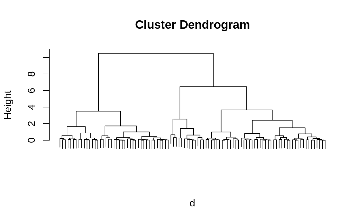
Figure 13.2: Hierarchical cluster dendrogram
Figure 13.2 allows us to now extract the three largest clusters. Obviously, we have a huge advantage here because we know the true number of clusters. Real life is rarely that easy. However, even if we didn’t already know we were dealing with three clusters, looking at the dendrogram gives us a good clue that there are three big clusters in the data.
clust is a vector of integers between 1 and 3, one integer for each
observation in the sample, that assigns each observation to a cluster.
Here are the first 20 cluster assignments:
By treating the cluster number as a factor, we can compute the mean of each statistical cluster (see Recipe 6.6), “Applying a Function to Groups of Data”):
R did a good job of splitting data into clusters: the means appear distinct, with one near –2.7, one near 0.27, and one near +3.2. (The order of the extracted means does not necessarily match the order of the original groups, of course.) The extracted means are similar but not identical to the original means. Side-by-side boxplots can show why:
library(patchwork)

df_cluster <- data.frame(x,
                         means = factor(means),
                         clust = factor(clust))

g1 <- ggplot(df_cluster) +
  geom_boxplot(aes(means, x)) +
  labs(title = "Original Clusters", x = "Cluster Mean")

g2 <- ggplot(df_cluster) +
  geom_boxplot(aes(clust, x)) +
  labs(title = "Identified Clusters", x = "Cluster Number")

g1 + g2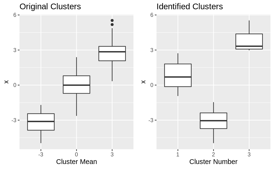
Figure 13.3: Cluster boxplots
The boxplots are shown in Figure 13.3. The clustering algorithm perfectly separated the data into nonoverlapping groups. The original clusters overlapped, whereas the identified clusters do not.
This illustration used one-dimensional data, but the dist function
works equally well on multidimensional data stored in a data frame or
matrix. Each row in the data frame or matrix is treated as one
observation in a multidimensional space, and dist computes the
distances between those observations.
See Also
This demonstration is based on the clustering features of the base
package. There are other packages, such as mclust, that offer
alternative clustering mechanisms.
13.7 Predicting a Binary-Valued Variable (Logistic Regression)
Problem
You want to perform logistic regression, a regression model that predicts the probability of a binary event occurring.
Solution
Call the glm function with family = binomial to perform logistic
regression. The result is a model object:
Here, b is a factor with two levels (e.g., TRUE and FALSE, 0 and
1), while x1, x2, and x3 are predictor variables.
Use the model object, m, and the predict function to predict a
probability from new data:
Discussion
Predicting a binary-valued outcome is a common problem in modeling. Will a treatment be effective or not? Will prices rise or fall? Who will win the game, team A or team B? Logistic regression is useful for modeling these situations. In the true spirit of statistics, it does not simply give a “thumbs up” or “thumbs down” answer; rather, it computes a probability for each of the two possible outcomes.
In the call to predict, we set type = "response" so that predict
returns a probability. Otherwise, it returns log-odds, which most of us don’t
find intuitive.
In his unpublished book entitled Practical Regression and ANOVA Using R,
Julian Faraway gives an example of predicting a binary-valued variable: test
from the dataset pima is true if the patient tested positive for
diabetes. The predictors are diastolic blood pressure and body mass
index (BMI). Faraway uses linear regression, so let’s try logistic
regression instead:
data(pima, package = "faraway")
b <- factor(pima$test)
m <- glm(b ~ diastolic + bmi, family = binomial, data = pima)
The summary of the resulting model, m, shows that the respective
p-values for the diastolic and the bmi variables are 0.8 and
(essentially) zero. We can therefore conclude that only the bmi
variable is significant:
summary(m)
#>
#> Call:
#> glm(formula = b ~ diastolic + bmi, family = binomial, data = pima)
#>
#> Deviance Residuals:
#>    Min      1Q  Median      3Q     Max
#> -1.913  -0.918  -0.685   1.234   2.742
#>
#> Coefficients:
#>             Estimate Std. Error z value Pr(>|z|)
#> (Intercept) -3.62955    0.46818   -7.75  9.0e-15 ***
#> diastolic   -0.00110    0.00443   -0.25      0.8
#> bmi          0.09413    0.01230    7.65  1.9e-14 ***
#> ---
#> Signif. codes:  0 '***' 0.001 '**' 0.01 '*' 0.05 '.' 0.1 ' ' 1
#>
#> (Dispersion parameter for binomial family taken to be 1)
#>
#>     Null deviance: 993.48  on 767  degrees of freedom
#> Residual deviance: 920.65  on 765  degrees of freedom
#> AIC: 926.7
#>
#> Number of Fisher Scoring iterations: 4
Because only the bmi variable is significant, we can create a reduced
model like this:
Let’s use the model to calculate the probability that someone with an average BMI (32.0) will test positive for diabetes:
newdata <- data.frame(bmi = 32.0)
predict(m.red, type = "response", newdata = newdata)
#>     1
#> 0.333
According to this model, the probability is about 33.3%. The same calculation for someone in the 90th percentile gives a probability of 54.9%:
See Also
Using logistic regression involves interpreting the deviance to judge the significance of the model. We suggest you review a text on logistic regression before attempting to draw any conclusions from your regression.
13.8 Bootstrapping a Statistic
Problem
You have a dataset and a function to calculate a statistic from that dataset. You want to estimate a confidence interval for the statistic.
Solution
Use the boot package. Apply the boot function to calculate bootstrap
replicates of the statistic:
library(boot)
bootfun <- function(data, indices) {
  # . . . calculate statistic using data[indices]. . .
  return(statistic)
}

reps <- boot(data, bootfun, R = 999)
Here, data is your original dataset, which can be stored in either a
vector or a data frame. The statistic function (bootfun in this case)
should expect two arguments: data is the original dataset, and
indices is a vector of integers that selects the bootstrap sample from
data.
Next, use the boot.ci function to estimate a confidence interval from
the replications:
Discussion
Anybody can calculate a statistic, but that’s just the point estimate.
We want to take it to the next level: What is the confidence interval (CI)?
For some statistics, we can calculate the CI analytically. The CI for a mean, for instance, is
calculated by the t.test function. Unfortunately, that is the
exception and not the rule. For most statistics, the mathematics is too
tortuous or simply unknown, and there is no known closed-form
calculation for the CI.
The bootstrap algorithm can estimate a CI even when no closed-form calculation is available. It works like this. The algorithm assumes that you have a sample of size N and a function to calculate the statistic:
Randomly select N elements from the sample, sampling with replacement. That set of elements is called a bootstrap sample.
Apply the function to the bootstrap sample to calculate the statistic. That value is called a bootstrap replication.
Repeat steps 1 and 2 many times to yield many (typically thousands) of bootstrap replications.
From the bootstrap replications, compute the confidence interval.
That last step may seem mysterious, but there are several algorithms for computing the CI. A simple one uses percentiles of the replications, such as taking the 2.5 percentile and the 97.5 percentile to form the 95% CI.
We’re huge fans of the bootstrap because we work daily with obscure statistics, it is important that we know their confidence interval, and there is definitely no known formula for their CI. The bootstrap gives us a good approximation.
Let’s work an example. In Recipe 13.4, “Performing Principal Component Analysis” we estimated the slope of a line using orthogonal regression. That gave us a point estimate, but how can we find the CI? First, we encapsulate the slope calculation within a function:
stat <- function(data, indices) {
  r <- prcomp(~ x + y, data = data, subset = indices)
  slope <- r$rotation[2, 1] / r$rotation[1, 1]
  return(slope)
}
Notice that the function is careful to select the subset defined by indices and to compute the slope from that exact subset.
Next, we calculate 999 replications of the slope. Recall that we had two vectors, x and y, in the original recipe; here, we combine them into a data frame:
load(file = './data/pca.rdata')
library(boot)
set.seed(3) # for reproducability

boot.data <- data.frame(x = x, y = y)
reps <- boot(boot.data, stat, R = 999)
The choice of 999 replications is a good starting point. You can always repeat the bootstrap with more and see if the results change significantly.
The boot.ci function can estimate the CI from the replications. It
implements several different algorithms, and the type argument selects
which algorithms are performed. For each selected algorithm, boot.ci
will return the resulting estimate:
boot.ci(reps, type = c("perc", "bca"))
#> BOOTSTRAP CONFIDENCE INTERVAL CALCULATIONS
#> Based on 999 bootstrap replicates
#>
#> CALL :
#> boot.ci(boot.out = reps, type = c("perc", "bca"))
#>
#> Intervals :
#> Level     Percentile            BCa
#> 95%   ( 1.03,  2.07 )   ( 1.06,  2.10 )
#> Calculations and Intervals on Original Scale
Here we chose two algorithms, percentile and BCa, by setting
type = c("perc","bca"). The two resulting estimates appear at the bottom
under their names. Other algorithms are available; see the help page for boot.ci.
You will note that the two confidence intervals are slightly different: (1.068, 1.992) versus (1.086, 2.050). This is an uncomfortable but inevitable result of using two different algorithms. We don’t know any method for deciding which is better. If the selection is a critical issue, you will need to study the reference and understand the differences. In the meantime, our best advice is to be conservative and use the minimum lower bound and the maximum upper bound; in this case, that would be (1.068, 2.050).
By default, boot.ci estimates a 95% CI. You can
change that via the conf argument, like this:
See Also
See Recipe 13.4, “Performing Principal Component Analysis” for the slope calculation. A good tutorial and reference for the bootstrap algorithm is An Introduction to the Bootstrap by Bradley Efron and Robert Tibshirani (Chapman & Hall/CRC).
13.9 Factor Analysis
Problem
You want to perform factor analysis on your dataset, usually to discover what your variables have in common.
Solution
Use the factanal function, which requires your dataset and your
estimate of the number of factors:
The output includes n factors, showing the loadings of each input variable for each factor.
The output also includes a p-value. Conventionally, a p-value of less than 0.05 indicates that the number of factors is too small and does not capture the full dimensionality of the dataset; a p-value exceeding 0.05 indicates that there are likely enough (or more than enough) factors.
Discussion
Factor analysis creates linear combinations of your variables, called factors, that abstract the variable’s underlying commonality. If your N variables are perfectly independent, then they have nothing in common and N factors are required to describe them. But to the extent that the variables have an underlying commonality, fewer factors capture most of the variance and so fewer than N factors are required.
For each factor and variable, we calculate the correlation between them, known as the loading. Variables with a high loading are well explained by the factor. We can square the loading to know what fraction of the variable’s total variance is explained by the factor.
Factor analysis is useful when it shows that a few factors capture most of the variance of your variables. Thus, it alerts you to redundancy in your data. In that case you can reduce your dataset by combining closely related variables or by eliminating redundant variables altogether.
A more subtle application of factor analysis is interpreting the factors to find interrelationships between your variables. If two variables both have large loadings for the same factor, then you know they have something in common. What is it? There is no mechanical answer. You’ll need to study the data and its meaning.
There are two tricky aspects of factor analysis. The first is choosing the number of factors. Fortunately, you can use PCA to get a good initial estimate of the number of factors. The second tricky aspect is interpreting the factors themselves.
Let’s illustrate factor analysis by using stock prices or, more precisely, changes in stock prices. The dataset contains six months of price changes for the stocks of 12 companies. Every company is involved in the petroleum and gasoline industry. Their stock prices probably move together, since they are subject to similar economic and market forces. We might ask: How many factors are required to explain their changes? If only one factor is required, then all the stocks are the same and one is as good as another. If many factors are required, we know that owning several of them provides diversification.
We start by doing a PCA on diffs, the data
frame of price changes. Plotting the PCA results shows the variance
captured by the components:
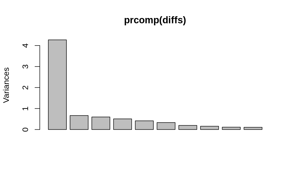
Figure 13.4: PCA results plot
We can see in Figure 13.4 that the first component captures much of the variance, but we don’t know if more components are required. So we perform the initial factor analysis while assuming that two factors are required:
factanal(diffs, factors = 2)
#>
#> Call:
#> factanal(x = diffs, factors = 2)
#>
#> Uniquenesses:
#>   APC    BP   BRY   CVX   HES   MRO   NBL   OXY   ETP   VLO   XOM
#> 0.307 0.652 0.997 0.308 0.440 0.358 0.363 0.556 0.902 0.786 0.285
#>
#> Loadings:
#>     Factor1 Factor2
#> APC 0.773   0.309
#> BP  0.317   0.497
#> BRY
#> CVX 0.439   0.707
#> HES 0.640   0.389
#> MRO 0.707   0.377
#> NBL 0.749   0.276
#> OXY 0.562   0.358
#> ETP 0.283   0.134
#> VLO 0.303   0.350
#> XOM 0.355   0.767
#>
#>                Factor1 Factor2
#> SS loadings       2.98   2.072
#> Proportion Var    0.27   0.188
#> Cumulative Var    0.27   0.459
#>
#> Test of the hypothesis that 2 factors are sufficient.
#> The chi square statistic is 62.9 on 34 degrees of freedom.
#> The p-value is 0.00184
We can ignore most of the output because the p-value at the bottom is very close to zero (.00184). The small p-value indicates that two factors are insufficient, so the analysis isn’t good. More are required, so we try again with three factors instead:
factanal(diffs, factors = 3)
#>
#> Call:
#> factanal(x = diffs, factors = 3)
#>
#> Uniquenesses:
#>   APC    BP   BRY   CVX   HES   MRO   NBL   OXY   ETP   VLO   XOM
#> 0.316 0.650 0.984 0.315 0.374 0.355 0.346 0.521 0.723 0.605 0.271
#>
#> Loadings:
#>     Factor1 Factor2 Factor3
#> APC  0.747   0.270   0.230
#> BP   0.298   0.459   0.224
#> BRY                  0.123
#> CVX  0.442   0.672   0.197
#> HES  0.589   0.299   0.434
#> MRO  0.703   0.350   0.167
#> NBL  0.760   0.249   0.124
#> OXY  0.592   0.357
#> ETP  0.194           0.489
#> VLO  0.198   0.264   0.535
#> XOM  0.355   0.753   0.190
#>
#>                Factor1 Factor2 Factor3
#> SS loadings      2.814   1.774   0.951
#> Proportion Var   0.256   0.161   0.086
#> Cumulative Var   0.256   0.417   0.504
#>
#> Test of the hypothesis that 3 factors are sufficient.
#> The chi square statistic is 30.2 on 25 degrees of freedom.
#> The p-value is 0.218
The large p-value (0.218) confirms that three factors are sufficient, so we can use the analysis.
The output includes a table of explained variance, shown here:
               Factor1 Factor2 Factor3
SS loadings      2.814   1.774   0.951
Proportion Var   0.256   0.161   0.086
Cumulative Var   0.256   0.417   0.504
This table shows that the proportion of variance explained by each factor is 0.256, 0.161, and 0.086, respectively. Cumulatively, they explain 0.504 of the variance, which leaves 1 – 0.504 = 0.496 unexplained.
Next we want to interpret the factors, which is more like voodoo than science. Let’s look at the loadings, repeated here:
Loadings:
    Factor1 Factor2 Factor3
APC  0.747   0.270   0.230
BP   0.298   0.459   0.224
BRY                  0.123
CVX  0.442   0.672   0.197
HES  0.589   0.299   0.434
MRO  0.703   0.350   0.167
NBL  0.760   0.249   0.124
OXY  0.592   0.357
ETP  0.194           0.489
VLO  0.198   0.264   0.535
XOM  0.355   0.753   0.190
Each row is labeled with the variable name (stock symbol): APC, BP, BRY, and so forth. The first factor has many large loadings, indicating that it explains the variance of many stocks. This is a common phenomenon in factor analysis. We are often looking at related variables, and the first factor captures their most basic relationship. In this example, we are dealing with stocks, and most stocks move together in concert with the broad market. That’s probably captured by the first factor.
The second factor is more subtle. Notice that the loadings for CVX (0.67) and XOM (0.75) are the dominant ones, with BP not far behind (0.46), but all other stocks have noticeably smaller loadings. This indicates a connection between CVX, XOM, and BP. Perhaps they operate together in a common market (e.g., multinational energy) and so tend to move together.
The third factor also has three dominant loadings: VLO, ETP, and HES. These are somewhat smaller companies than the global giants we see in the first factor. Possibly these three share similar markets or risks and so their stocks also tend to move together.
In summary, it seems there are three groups of stocks here:
CVX, XOM, BP
VLO, ETP, HES
Everything else
Factor analysis is an art and a science. We suggest that you read a good book on multivariate analysis before employing it.
See Also
See Recipe 13.4, “Performing Principal Component Analysis”, for more about PCA.